

Support Vector Machine

• Support vector machine (SVM) is a binary linear classifier

• There are tricks to make SVM able to solve non-linear problems

• There are extensions which allows using SVM to multiclass classification or regression

• SVM is a supervised learning algorithm

• There are extensions which allows using SVM for (unsupervised) clustering

Linear SVM

• Lets consider a training dataset of $N$ samples $(\vec x_1, y_1), \cdots, (\vec x_N, y_N)$

• $\vec x_i$ is $D$-dimensional vector representing features

• $y_i$ is a class label, for convenience $y_i = \left\{-1, 1\right\}$

• At this point we assume that classes are linearly separable

• For visualization purpose lets use $D = 2$

# our standard imports: matplotlib and numpy
import matplotlib.pyplot as plt
import numpy as np

# just to overwrite default colab style
plt.style.use('default')
plt.style.use('seaborn-talk')

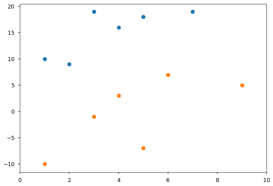
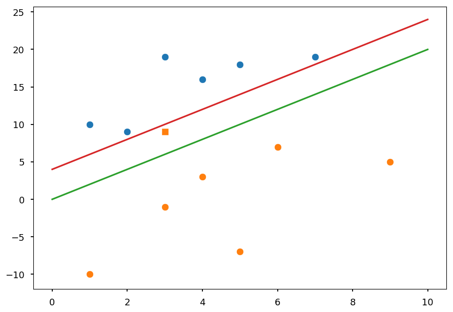
# class I
X01 = [(2, 9), (7, 19), (1, 10), (3, 19), (4, 16), (5, 18)]

# class II
X02 = [(4, 3), (6, 7), (1, -10), (3, -1), (9, 5), (5, -7)]

plt.xlim([0, 10])

plt.scatter(*(zip(*X01)))
plt.scatter(*(zip(*X02)));

• In general we want to find a hyperplane which separates two classes

• In the example above is just a line

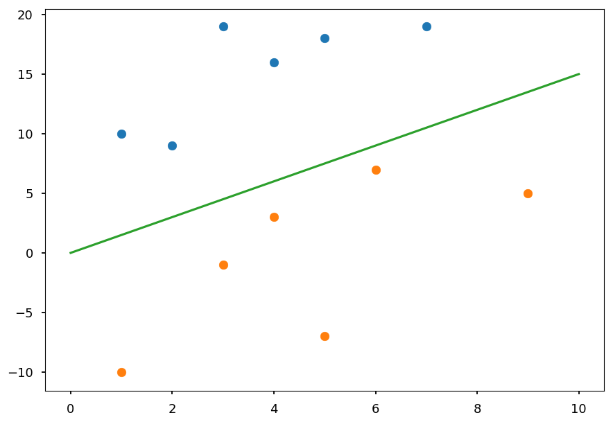
plt.scatter(*(zip(*X01)))
plt.scatter(*(zip(*X02)))

plt.plot([0, 10], [0, 15], 'C2-');

• Once a hyperplane is found, the classification is straightforward

• In this case, everything above a line is classified as a blue point and below as an orange point

• However, there is infinitely many possible lines / hyperplanes

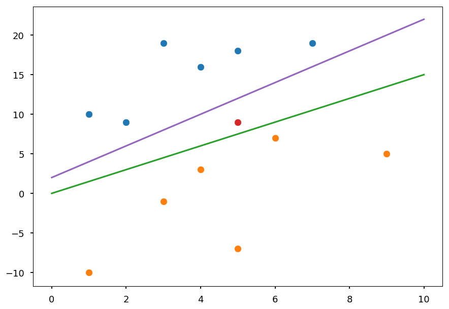
plt.scatter(*(zip(*X01)))
plt.scatter(*(zip(*X02)))

plt.scatter(5, 9, c='C3')  # test point

plt.plot([0, 10], [2, 22], 'C4-');
plt.plot([0, 10], [0, 15], 'C2-');

• On the plot above two possible lines which correctly classify all training data are drawn

• The red point represents a test sample

• Using "by eye" method one could say it is rather orange than blue

• The final predictions depends on the choice of a line though

• Thus, one need a criterion to choose the best line / hyperplane

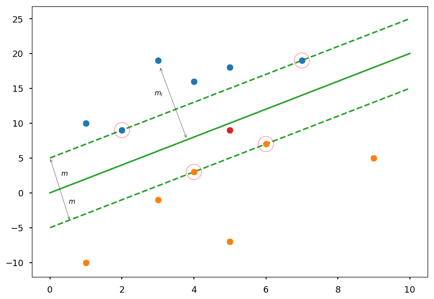
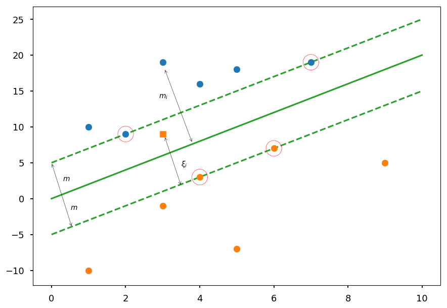
• SVM chooses the hyperplane which is maximally far away from any training point

plt.plot([0, 10], [0, 20], 'C2-', zorder=0)
plt.plot([0, 10], [5, 25], 'C2--', zorder=0)
plt.plot([0, 10], [-5, 15], 'C2--', zorder=0)

plt.scatter(5, 9, c='C3')  # test point

plt.annotate('', (0,5), (0.55, -4), arrowprops=dict(arrowstyle='<->'))
plt.text(0.5, -1.5, '$m$')
plt.text(0.3, 2.5, '$m$')

plt.annotate('', (3.05,18.1), (3.8, 7.75), arrowprops=dict(arrowstyle='<->'))
plt.text(2.9, 14, '$m_i$')

plt.scatter(*(zip(*X01)), zorder=1)
plt.scatter(*(zip(*X02)), zorder=1)

sv = X01[:2] + X02[:2]

plt.scatter(*(zip(*sv)), zorder=1, facecolors='none', edgecolors='r', s=500);

• The goal is to maximize the margin $2m$

• Please note, that the margin is given by the distance of closest data point to the hyperplane

• Which means, that the classifier depends only on a small subset of training data, which are called support vectors

Hard margin

• Any hyperplane can be defined by an intercept term $b$ and a normal vector $\vec w$ (which is usually called weights in machine learning)

• All the points $\vec x$ on the hyperplane satisfy $\vec w \cdot \vec x + b = 0$

• If $\vec w \cdot \vec x + b~{> \choose <}~0$ the point is on the $\text{one} \choose \text{other}$ side

• We can easily defined the linear classifier

  
  $f(\vec x) = \text{sign}\left(\vec w \cdot \vec x + b\right)$

  
  

• That is why we wanted class labels to be $-1$ or $1$ (instead more standard $0$ and $1$)

• All we need is to find weights

Functional margin

• Lets define functional margin of hyperplane $(\vec w, b)$ w.r.t. a training sample $(\vec x_i, y_i)$ as

  
  $\hat m_i = y_i\cdot \left(\vec w \cdot \vec x_i + b\right)$

  
  

• It is only positive if the training sample label has the same sign as prediction

• The magnitude tells us somewhat about the confidence of a prediction

• But please note, that we can choose arbitrary factor $k$ and $\text{sign}\left(\vec w \cdot \vec x + b\right) = \text{sign}\left(k\cdot\vec w \cdot \vec x + k\cdot b\right)$

• Function margin w.r.t. the whole training dataset is the smallest one

  
  $\hat m = \min\limits_{i = 1, \cdots, N}\hat m_i$

  
  

Geometric margin

• Lets $m_i$ be a distance from a training point $\vec x_i$ to a decision boundary / hyperplane $(\vec w, b)$

• Lets $\vec x_h$ be a point on a hyperplane closest to $\vec x_i$

• Shortest distance must be peprendicular to a hyperplane (so parallel to $\vec w$)

• We can express $\vec x_h$ by

  
  $\vec x_h = \vec x_i - y_i\cdot m_i\cdot \frac{\vec w}{|\vec w|}$

  
  

• Because $\vec x_h$ lies on a hyperplane it must fulfill $\vec w \cdot \vec x_h + b = 0$, thus

  
  $\vec w\left(\vec x_i - y_i\cdot m_i\cdot \frac{\vec w}{|\vec w|}\right) + b = 0$

  
  

• Pretty straightforward to solve for $m_i$

  
  $m_i = y_i\frac{\vec w\cdot \vec x_i + b}{|\vec w|} = \frac{\hat m_i}{|\vec w|}$

  
  

• As before geometric margin w.r.t. the whole training dataset is the smallest one

  
  $m = \min\limits_{i = 1, \cdots, N} m_i = \frac{\hat m}{|\vec w|}$

  
  

• Please note, that $m$ does not change when weights are scaled

• $\hat m = m$ for $|\vec w| = 1$

The optimal margin

• We want to find the maximum geometric margin $m$

• But with a constraint that for every sample outside the margin

  
  $\left.\begin{array}{cc}\text{maximize}_{w, b, m} & m\\\text{subject to} & m_i \geq m\end{array}\right.$

  
  

• As we discussed, we can choose any normalization of normal vector $|\vec w|$ as it does not change the value of $m_i = y_i\frac{\vec w\cdot \vec x_i + b}{|\vec w|}$

• Lets choose $|\vec w| = \frac{1}{m}$, so

  
  $\left.\begin{array}{cc}\text{maximize}_{w, b} & \frac{1}{|\vec w|}\\\text{subject to} & |\vec w|\cdot m_i \geq 1\end{array}\right.$

  
  

• Since maximizing $|\vec w|^{-1}$ means the same as minimizing $|\vec w|$, we can finally write

  
  $\left.\begin{array}{cc}\text{minimize}_{w,b} & \frac{1}{2}|\vec w|^2\\\text{subject to} & \hat m_i \geq 1\end{array}\right.$

  
  

• Please note that we choose $|\vec w|^2$ over $|\vec w|$ to avoid square root, and $\frac{1}{2}$ is for math convenience

• Now, all we need is to optimize quadratic function over variables subject to linear constraints (quadratic programming)

Lagrange multipliers

• Lagrange multipliers is the common method used to solve contrained optimization problems

• Lets consider the following problem (with equality constraint):

  
  $\left.\begin{array}{cc}\text{minimize} & f(\vec x)\\\text{subject to} & g(\vec x) = 0\end{array}\right.$

  
  

• Please note, that one could also consider $g(\vec x) = c$, where $c$ is constant (then $g'(\vec x) = g(\vec x) - c = 0$)

• Lagrange multiplier theorem says that at constrained optimum (if exists) $\nabla f$ will be parallel to $\nabla g$, so

  
  $\nabla f(\vec x) = \lambda\nabla g(\vec x)$

  
  

• $\lambda$ - a Lagrange multiplier

How it works

• Lets consider the following problem:

  
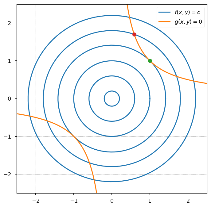
  $\left.\begin{array}{cc}\text{minimize} & f(x, y) = x^2 + y^2\\\text{subject to} & g(x, y) = x\cdot y - 1 = 0\end{array}\right.$

  
  

def flc(c, n=100):
  """Level curves of objective functions"""
  return np.array([(c * np.cos(ang), c * np.sin(ang))
                   for ang in np.linspace(0, 2*np.pi, n)])

def g(n=100):
  """Constraint"""
  return np.array([(x, 1./x) for x in np.linspace(0.1, 2.5, n)])

##### PLOT SETTINGS #####

plt.figure(figsize=(8, 8))
plt.xlim([-2.5, 2.5])
plt.ylim([-2.5, 2.5])
plt.grid(color='0.5', linestyle='--', linewidth=0.5)

##### LEVEL CURVES OF f(x, y) #####

for c in (0.2, 0.6, 1, 1.8, 2.2):
  plt.plot(*flc(c).T, color='C0')

plt.plot(*flc(np.sqrt(2)).T, color='C0', label='$f(x, y) = c$')

##### CONSTRAINTS #####

plt.plot(*g().T, color='C1', label='$g(x, y) = 0$')
plt.plot(*-g().T, color='C1')

##### INTERSECTIONS #####

plt.scatter(1, 1, c='C2', zorder=4)
plt.scatter(np.sqrt(0.345), np.sqrt(1/0.345), c='C3', zorder=4)

plt.legend();

• Blue lines represent the level curves of the objective function ($f(x, y) = const$)

• Orange lines represent the constraints ($g(x, y) = 0$)

• Lets first consider the case that blue and orange curves are not tangent (red point)

  • going along the constraint one direction would result in the decrease of the objective function

  • while going in another direction would result in the increase of the objective function

  • thus, this point can not be an optimum

• The only possibility is that a constrained optimum is where curves are tanget (it still may not be the case, but at least it could be)

Lagrangian

• In general, there may be many constraints:

  
  $\left.\begin{array}{cc}\text{minimize} & f(\vec x)\\\text{subject to} & g_i(\vec x) = 0, \hspace{5pt} i = 0,\cdots, M\end{array}\right.$

  
  

• Then, there are $M$ Lagrange multipliers $\lambda_i$

• It is convenient to define Lagrangian:

  
  $\mathcal{L}(\vec x, \lambda) = f(\vec x) + \sum\limits_{i=1}^M\lambda_ig_i(\vec x)$

  
  

• and solve:

  
  $\nabla_{x_1,\cdots, x_n, \lambda_1,\cdots, \lambda_M} \mathcal{L}(\vec x, \lambda) = 0$

  
  

• which is equivalent to:

  
  $\nabla f(\vec x) = \sum\limits_{i=1}^M\lambda_i\nabla g_i(\vec x)$
  $g_1(\vec x) = \cdots = g_M(\vec x) = 0$

  
  

• The optimum (if exists) is always a saddle point of the Lagrangian

  • On the one hand, we want to minimize the Lagrangian over $\vec x$

  • And on the other hand, we want to maximize the Lagrangian over $\lambda_i$

Example

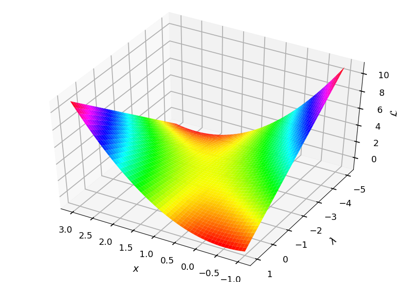
• Lets consider the objective function $f(x) = x^2$ with a constraint $g(x) = x - 1 = 0$

• The Lagrangian is given by:

  
  $\mathcal{L}(x, \lambda) = x^2 + \lambda\cdot (x - 1)$
  $\frac{\partial\mathcal{L}}{\partial x} = 2x + \lambda = 0$
  $\frac{\partial\mathcal{L}}{\partial\lambda} = x - 1 = 0$

  
  

• It has a saddle point at $x = 1$ and $p = -2$

from mpl_toolkits.mplot3d import Axes3D
from matplotlib import cm

ax = plt.figure().add_subplot(111, projection=Axes3D.name)

X, Y = np.meshgrid(np.linspace(-1, 3, 50), np.linspace(-5, 1, 50))
L = X**2 + Y * (X - 1)

ax.plot_surface(X, Y, L, cmap=cm.hsv)

ax.view_init(elev=45, azim=120)

ax.set_xlabel('$x$', labelpad=20)
ax.set_ylabel('$\lambda$', labelpad=20)
ax.set_zlabel('$\mathcal{L}$', labelpad=10);

Lagrange duality

• Lets consider the optimization problem with inequality constraints:

  
  $\left.\begin{array}{cc}\text{minimize} & f(\vec x)\\\text{subject to} & g_i(\vec x) \leq 0, \hspace{5pt} i = 0,\cdots, M\\\text{} & h_i(\vec x) = 0, \hspace{5pt} i = 0,\cdots, N\end{array}\right.$

  
  

• We will call it the primal optimization problem and define generalized Lagrangian:

  
  $\mathcal{L}(\vec x, \mu, \lambda) = f(\vec x) + \sum\limits_{i=1}^M\mu_ig_i(\vec x) + \sum\limits_{i=1}^N\lambda_ih_i(\vec x)$

  
  

• with the additional restriction that $\mu_i \geq 0$

  • if $i$-th constraint is fulfilled, making $\mu_i$ more positive decrease the Lagrangian

  • making $\mu_i$ negative is not allowed

• Please note, that in the case of constraints $g_i \geq 0$, the restriction is $\mu_i \leq 0$

• The task can be expressed in terms of minimizing the following function:

  
  $\theta_P(\vec x) = \left\{\begin{array}{cc}f(\vec x) & \text{if x satisfies primal constraints} \\ \infty & \text{otherwise}\end{array}\right. = \max\limits_{\mu, \lambda; \mu_i \geq 0}\mathcal{L}(\vec x, \mu, \lambda)$

  
  

• Thus, we can write the final task in the form:

  
  $\min\limits_{\vec x}\theta_P(\vec x) = \min\limits_{\vec x}\max\limits_{\mu, \lambda; \mu_i \geq 0}\mathcal{L}(\vec x, \mu, \lambda)$

  
  

• Now, lets consider the following "reversed" task:

  
  $\max\limits_{\mu, \lambda; \mu_i \geq 0}\min\limits_{\vec x}\mathcal{L}(\vec x, \mu, \lambda) = \max\limits_{\mu, \lambda; \mu_i \geq 0}\theta_D(\mu, \lambda)$

  
  

• $\theta_D(\mu, \lambda)$ is known as the dual function and the maximizing it is called the dual problem

• $\theta_D(\mu, \lambda)$ is a concave function (becasue Lagrangian is affine, i.e. linear in multipliers) - maximing $\theta_D$ is a convex optimisation problem

• How it is related to the primal problem:

  
  $\mathcal{L}(\vec x, \mu, \lambda) \leq \theta_P(\vec x)$
  
  $\min\limits_{\vec x}\mathcal{L}(\vec x, \mu, \lambda) = \theta_D(\mu, \lambda) \leq \min\limits_{\vec x}\theta_P(\vec x)\equiv p^*$
  
  $d^* \equiv \max\limits_{\mu, \lambda; \mu_i \geq 0}\theta_D(\mu, \lambda) \leq p^*$

  
  

• Thus, the optimum of the dual problem $d^*$ is a lower bound for the optimum of the primal problem $p^*$ (known as weak duality)

• The difference $p^* - d^*$ is known as the duality gap

• If the gap is zero ($p^* = d^*$) we have strong duality

• If the optimization problem is convex and (strictly) feasible (i.e. there is $\vec x$ which satisfies all constraints) strong duality holds, so there must exist $\vec x^*$, $\mu^*$, $\lambda^*$, so that $\vec x^*$ is the solution of the primal problem and $\mu^*$ and $\lambda^*$ are solutions of the dual problem, and

  
  $p^* = d^* = \mathcal{L}(\vec x^*, \mu^*, \lambda^*)$

  
  

KKT conditions

• Moreover, $\vec x^*$, $\mu^*$, $\lambda^*$ satisfy the Karush-Kuhn-Tucker (KKT) conditions

• Stationarity

  
  $\nabla_{\vec x} \mathcal{L}(\vec x^*, \mu^*, \lambda^*) = 0$

  
  

• Primal feasibility

  
  $g_i(\vec x^*) \leq 0, \hspace{10pt} h_i(\vec x^*) = 0$

  
  

• Dual feasibility

  
  $\mu_i^* \geq 0$

  
  

• Complementary slackness (or dual complementarity)

  
  $\mu_i^*\cdot g_i(\vec x^*) = 0$

  
  

• Why the last one - for strong duality:

  
  $f(\vec x^*) = \theta_D(\mu^*, \lambda^*) = \min\limits_{\vec x}\mathcal{L}(\vec x, \mu^*, \lambda^*) \leq f(\vec x^*) + \sum\limits_{i=1}^M\mu_i^*\cdot g_i(\vec x^*) + \sum\limits_{i=1}^N\lambda_i^*\cdot h_i(\vec x ^*) \leq f(\vec x^*)$

  
  

• The last inequality holds beacause $\sum\limits_{i=1}^M\mu_i^*\cdot g_i(\vec x^*) \leq 0$

• Since $f(\vec x^*)$ must be equal to $f(\vec x^*)$ these inequalities are in fact equalities, so $\sum\limits_{i=1}^M\mu_i^*\cdot g_i(\vec x^*) = 0$

• Because $\mu_i \geq 0$ and $g_i \leq 0$ we get the complementary slackness condition: $\mu_i^*\cdot g_i(\vec x^*) = 0$

• If $\vec x^*$, $\mu^*$, $\lambda^*$ satisfy KKT conditions, then they are primal and dual solutions

Optimal margin

• Lets back to our original optimization problem:

  
  $\left.\begin{array}{cc}\text{minimize}_{w,b} & \frac{1}{2}|\vec w|^2\\\text{subject to} & y_i\cdot \left(\vec w \cdot \vec x_i + b\right) \geq 1\end{array}\right.$

  
  

• Lets rewrite the constraints in the form: $g_i(\vec w) = - y_i\cdot \left(\vec w \cdot \vec x_i + b\right) + 1 \leq 0$

• Please note, that because of the complementary slackness condition, $\mu_i > 0$ only for the training examples ($\vec x_i$) that have functional margin equal to one (support vectors)

• Lets write the Langrangian for this problem:

  
  $\mathcal{L}(\vec w, b, \mu) = \frac{1}{2}|\vec w|^2 - \sum\limits_{i=1}^M\mu_i\cdot \left[y_i\cdot\left(\vec w \cdot \vec x_i + b\right) - 1\right]$

  
  

Dual problem

• To find the dual form of the problem we need to minimize the Lagrangian over $\vec w$ and $b$:

  
  $\nabla_{w}\mathcal{L}(\vec w, b, \mu) = \vec w - \sum\limits_{i=1}^M\mu_iy_i\vec x_i = 0 \Rightarrow \vec w = \sum\limits_{i=1}^M\mu_iy_i\vec x_i$

  
  

• And for the intercept term:

  
  $\frac{\partial}{\partial b}\mathcal{L}(\vec w, b, \mu) = \sum\limits_{i=1}^M\mu_iy_i = 0$

  
  

• It is straightforawrd to show, that using two above equations one can obtain:

  
  $\nabla_{w}\mathcal{L}(\vec w, b, \mu) = \sum\limits_{i=1}^M\mu_i - \frac{1}{2}|\vec w|^2 = \sum\limits_{i=1}^M\mu_i - \frac{1}{2}\sum\limits_{i,j=1}^My_iy_j\mu_i\mu_j\cdot\left(\vec x_i\cdot \vec x_j\right)$

  
  

• By examing the dual form the optimization problem is expressed in terms of the inner product of input feature vectors:

  
  $\left.\begin{array}{cc}\text{maximize}_{\mu} & \sum\limits_{i=1}^M\mu_i - \frac{1}{2}\sum\limits_{i,j=1}^My_iy_j\mu_i\mu_j\cdot\left<\vec x_i, \vec x_j\right>\\\text{subject to} & \mu_i \geq 0 \\ & \sum\limits_{i=1}^M\mu_iy_i = 0\end{array}\right.$

  
  

Non-linear SVM

• SVM can be applied to non-linear problems using the kernel trick

• However, before we go there, lets consider a simple non-linear problem

Example

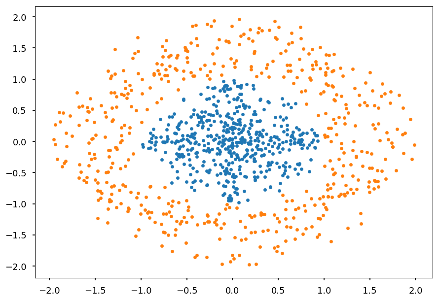
• Lets consider two classes of 2D points:

  • inside a circle

  • outside a circle

def generate_circle_data(R1=0, R2=1, N=500):
  """Generate N points in a circle for radius range (R1, R2)"""
  r = lambda: R1 + np.random.random() * (R2 - R1)

  return np.array([(r() * np.cos(ang), r() * np.sin(ang))
                   for ang in np.linspace(0, 2*np.pi, N)])

C01 = generate_circle_data()
C02 = generate_circle_data(1, 2)

plt.scatter(*C01.T, marker='.')
plt.scatter(*C02.T, marker='.');

• There is no way to find a line which separates these classes

• But would it be possible to add another dimension and find a plane?

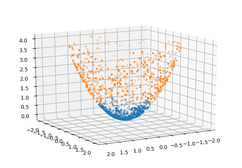
• Lets consider a feature mapping $\phi$ which maps original attributes:

  
  $\phi(x, y) = \left[\begin{array}{c} x \\ y \\ x^2 + y^2\end{array}\right]$

  
  

from mpl_toolkits.mplot3d import Axes3D
from matplotlib import cm

ax = plt.figure().add_subplot(111, projection=Axes3D.name)

Z01 = np.array([x**2 + y**2 for x, y in C01])
Z02 = np.array([x**2 + y**2 for x, y in C02])

ax.scatter(*C01.T, Z01, cmap=cm.hsv)
ax.scatter(*C02.T, Z02, cmap=cm.hsv)

ax.view_init(elev=15, azim=60)

• The new dataset is a linear problem and can be easily solved with SVM

• All we need is to replace (in the dual formulation): $\left<\vec x_i, \vec x_j\right> \rightarrow \left<\phi(\vec x_i), \phi(\vec x_j)\right> = \phi^T(\vec x_i)\phi(\vec x_j)$

Kernel trick

• Lets define the kernel (for given feature mapping $\phi$) as

  
  $K(\vec x_i, \vec x_j) = \phi^T(\vec x_i)\phi(\vec x_j)$

  
  

• Thus, the optimization problem we are trying to solve now is:

  
  $\left.\begin{array}{cc}\text{maximize}_{\mu} & \sum\limits_{i=1}^M\mu_i - \frac{1}{2}\sum\limits_{i,j=1}^My_iy_j\mu_i\mu_j\cdot K(\vec x_i, \vec x_j)\\\text{subject to} & \mu_i \geq 0 \\ & \sum\limits_{i=1}^M\mu_iy_i = 0\end{array}\right.$

  
  

• The trick is now, that we do not have to calculate (or even know) the mapping $\phi$, which could be in general very expensive

• The classifier was deinfed as:

  
  $\hat y = \text{sign}\left(\vec w \cdot \vec x + b\right)$

  
  

• and its dual form is:

  
  $\hat y = \text{sign}\left(\sum\limits_{i=1}^M \mu_iy_i\left<\vec x_i, \vec x\right> + b\right)$

  
  

• and can be now rewritten in the form:

  
  $\hat y = \text{sign}\left(\sum\limits_{i=1}^M \mu_iy_iK(\vec x_i, \vec x) + b\right)$

  
  

Example

• Lets consider the feature mapping $\phi$ (in 3D):

  
  $\phi(\vec x) = \left[\begin{array}{c} x_1x_1 \\ x_1x_2 \\ x_1x_3 \\ x_2x_1 \\ x_2x_2 \\ x_2x_3 \\ x_3x_1 \\ x_3x_2 \\ x_3x_3\end{array}\right]$

  
  

• Calculating $\phi(\vec x)$, where $\vec x \in \mathcal{R}^N$, requires $O(n^2)$ time

• The related kernel is given by:

  
  $K(\vec x_i, \vec x_j) = \left<x_i, \vec x_j\right>^2$

  
  

• requires only $O(n)$ time

Mercer theorem

• Having some function $K$, how can we tell if it is a valid kernel?

• For a valid kernel, there must exist a feature mapping $\phi$, so that $K(\vec x_i, \vec x_j) = \phi^T(\vec x_i)\phi(\vec x_j)$

• Lets define the kernel matrix $K_{ij} = K(\vec x_i, \vec x_j)$

• If $K$ is a valid kernel the corresponding matrix must be symmetric: $K_{ij} = \phi^T(\vec x_i)\phi(\vec x_j) = \phi^T(\vec x_j)\phi(\vec x_i) = K_{ji}$

• Moreover, $K$ must be positive semi-definite ($K \geq 0$):

  
  $z^TKz = \sum\limits_i\sum\limits_jz_iK_{ij}z_j = \sum\limits_i\sum\limits_jz_i\phi^T(\vec x_i)\phi(\vec x_j)z_j = \sum\limits_i\sum\limits_j\sum\limits_kz_i\phi_k(\vec x_i)\phi_k(\vec x_j)z_j = \sum\limits_k\left(\sum\limits_iz_i\phi_k(\vec x_i)\right)^2 \geq 0$

  
  

• Mercer theorem

Let $K: \mathcal{R}^n\times \mathcal{R}^N \rightarrow \mathcal{R}$ be given. Then, for $K$ to be a valid kernel, it is necessary and **sufficient** that for any $\left\{x_1, \cdots x_m\right\}$, the corresponding kernel matrix is symmetric positive semi-definite.

Kernel examples

• Gaussian kernel

  
  $K(\vec x, \vec y) = \exp\left(-\frac{||\vec x - \vec y||}{2\sigma^2}\right)$

  
  

• Polynomial kernel

  
  $K(\vec x, \vec y) = \left(\vec x \cdot \vec y + c\right)^d$

  
  

• Sigmoid kernel

  
  $K(\vec x, \vec y) = \tanh\left(a\vec x \cdot \vec y + c\right)$

  
  

Soft margin

• So far, everything was considered with the assumption that data is (linearly) separable

• Mapping to a high-dimensional feature space may make data separable, but it can not guarantee that

• Also, due to some noise in data, some outliers may lead to overfitting

• Lets consider the example below

plt.plot([0, 10], [0, 20], 'C2-', zorder=0)
plt.plot([0, 10], [4, 24], 'C3-', zorder=0)

plt.scatter(3, 9, c='C1', marker=',')

plt.scatter(*(zip(*X01)), zorder=1)
plt.scatter(*(zip(*X02)), zorder=1);

• The green line represents the optimal decision boundary if the orange square point is not included

• The red line represents the case when the outlier is considered

• Including the extra point drastically changes the result

• The idea behind the soft margin is to allow some points to lie of the wrong side of a decision boundary

plt.plot([0, 10], [0, 20], 'C2-', zorder=0)
plt.plot([0, 10], [5, 25], 'C2--', zorder=0)
plt.plot([0, 10], [-5, 15], 'C2--', zorder=0)

plt.scatter(3, 9, c='C1', marker=',')
plt.annotate('', (3.05,8.7), (3.5, 1.75), arrowprops=dict(arrowstyle='<->'))
plt.text(3.5, 4.5, '$\\xi_i$')

plt.annotate('', (0,5), (0.55, -4), arrowprops=dict(arrowstyle='<->'))
plt.text(0.5, -1.5, '$m$')
plt.text(0.3, 2.5, '$m$')

plt.annotate('', (3.05,18.1), (3.8, 7.75), arrowprops=dict(arrowstyle='<->'))
plt.text(2.9, 14, '$m_i$')

plt.scatter(*(zip(*X01)), zorder=1)
plt.scatter(*(zip(*X02)), zorder=1)

sv = X01[:2] + X02[:2]

plt.scatter(*(zip(*sv)), zorder=1, facecolors='none', edgecolors='r', s=500);

Regularization

• Regularization is a common technique to prevent overfitting (more about that next week)

• Lets reformulate the original optimization problem:

  
  $\left.\begin{array}{cc}\text{minimize}_{w,b} & \frac{1}{2}|\vec w|^2 + C\sum \limits_i\xi_i\\\text{subject to} & \hat y_i\cdot\left(\vec w \cdot \vec x + b\right) \geq 1 - \xi_i \\ & \xi_i \geq 0\end{array}\right.$

  
  

• We now allow to have a functional margin less than 1, but if a training point has functional margin $1 - \xi_i$ we would pay a cost of the objective function being increased by $C\xi_i$

• Thus, $C$ controls how much we penalize "bad" points (with $C = \infty$ we are back to the original perfectly separate case)

• Lets write the Lagrangian for this optimization problem:

  
  $\mathcal{L}(\vec w, b, \xi, \mu, r) = \frac{1}{2}|\vec w|^2 + C\sum \limits_{i=1}^M \xi_i - \sum\limits_{i=1}^M\mu_i\cdot \left[y_i\cdot\left(\vec w \cdot \vec x_i + b\right) - 1 + \xi_i\right] - \sum\limits_{i=1}^Mr_i\xi_i$

  
  

• After the same procedure as before we get similar dual problem:

  
  $\left.\begin{array}{cc}\text{maximize}_{\mu} & \sum\limits_{i=1}^M\mu_i - \frac{1}{2}\sum\limits_{i,j=1}^My_iy_j\mu_i\mu_j\cdot\left<\vec x_i, \vec x_j\right>\\\text{subject to} & C \geq \mu_i \geq 0 \\ & \sum\limits_{i=1}^M\mu_iy_i = 0\end{array}\right.$

  
  

• The only difference is the extra constraint on $\mu_i$, which comes from $\frac{\partial\mathcal{L}}{\partial\xi_i} = C - \mu_i - r_i = 0$

• Lets consider also complementary slackness conditions:

  
  $\mu_i\cdot\left[y_i\cdot\left(\vec w \cdot \vec x_i + b\right) - 1 + \xi_i\right] = 0$
  $r_i\xi_i = 0$

  
  

• In the case $\mu_i = 0$, $r_i = C > 0 \Rightarrow \xi_i = 0$:

  
  $y_i\cdot\left(\vec w \cdot \vec x + b\right) \geq 1$

  
  

• In the case $\mu_i = C$, $r_i = 0 \Rightarrow \xi_i \geq 0$:

  
  $y_i\cdot\left(\vec w \cdot \vec x + b\right) \leq 1$

  
  

• In the case $0 < \mu_i < C$, $r_i = C - \mu_i > 0 \Rightarrow \xi_i = 0$:

  
  $y_i\cdot\left(\vec w \cdot \vec x + b\right) = 1$

  
  

SMO algorithm

• We need to solve:

  
  $\left.\begin{array}{cc}\text{maximize}_{\mu} & \sum\limits_{i=1}^M\mu_i - \frac{1}{2}\sum\limits_{i,j=1}^My_iy_j\mu_i\mu_jk_{ij} \equiv \mathcal{L}_D(\mu)\\\text{subject to} & C \geq \mu_i \geq 0 \\ & \sum\limits_{i=1}^M\mu_iy_i = 0\end{array}\right.$

  
  

• where (for convenience) $k_{ij} = K(\vec x_i, \vec x_j)$

• Sequential minimal optimization (SMO) algorithm solves the smallest possible optimization problem at a time

• By updating two Lagrange multipliers $\mu_i$ in a step

• One can not update only one because of the constraint $\sum\limits_i\mu_iy_i = 0$

Quick math

• Without loss of generality, lets consider optimizing $\mu_1$ and $\mu_2$ from an old set of feasible solution: $\mu_1^{old}, \mu_2^{old}, \mu_3 \cdots \mu_M$

• Because of the constraint, $y_1\mu_1 + y_2\mu_2 = y_1\mu_1^{old} + y_2\mu_2^{old}$

• Which can be rewritten as:

  
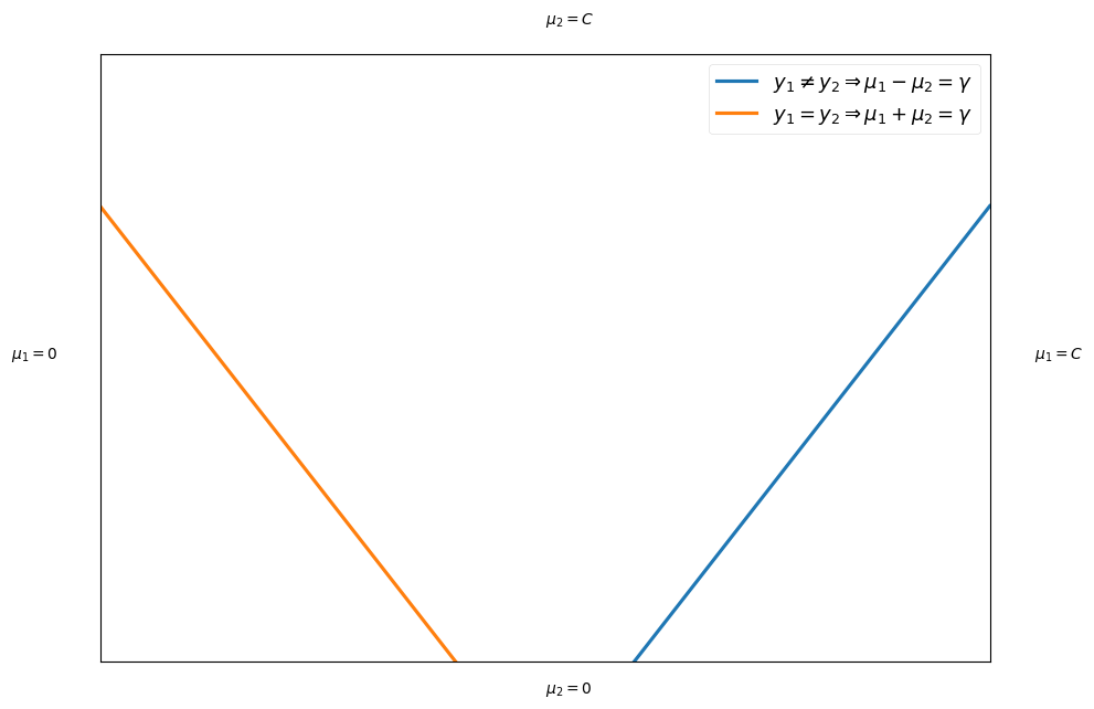
  $\mu_1 = \gamma - s\mu_2$

  
  

• where $s = y_1y_2$ and $\gamma = \mu_1 + s\mu_2 = \mu_1^{old} + s\mu_2^{old}$

• Thus, the optimization is on a line as shown below (two possibilities based on the sign of $s$):

plt.xticks([], [])
plt.yticks([], [])
plt.xlim([0,1])
plt.ylim([0,1])

plt.text(1.05, 0.5, "$\mu_1 = C$")
plt.text(-0.1, 0.5, "$\mu_1 = 0$")
plt.text(0.5, 1.05, "$\mu_2 = C$")
plt.text(0.5, -0.05, "$\mu_2 = 0$")

plt.plot((0.6,1), (0,0.75), label="$y_1 \\neq y_2 \Rightarrow \mu_1 - \mu_2 = \gamma$")
plt.plot((0.4,0), (0,0.75),  label="$y_1 = y_2 \Rightarrow \mu_1 + \mu_2 = \gamma$")

plt.legend();

• First lets fixed all $\mu_i$ for $i \neq 1,2$ and write the objective funtion in the following term:

$\begin{eqnarray} \mathcal{L}_D & = & \mu_1 + \mu_2 + const \\ & - & \frac{1}{2}\left(k_{11}\mu_1^2 + k_{22}\mu_2^2 + 2sk_{12}\mu_1\mu_2\right) \\ & - & y_1\mu_1\sum\limits_{i=3}^My_i\mu_ik_{1i} - y_2\mu_2\sum\limits_{i=3}^My_2\mu_2k_{2i} \\ & + & const \end{eqnarray}$

• Where $const$ does not depend on either $\mu_1$ nor $\mu_2$

• Please note, that when formulating the dual problem we got:

  
  $\nabla_{w}\mathcal{L}(\vec w, b, \mu) = \vec w - \sum\limits_{i=1}^M\mu_iy_i\vec x_i = 0 \Rightarrow \vec w = \sum\limits_{i=1}^M\mu_iy_i\vec x_i$

  
  

• For convenience, lets introduce:

$\begin{eqnarray} v _j & = & \sum\limits_{i=3}y_i\mu_ik_{ij} \\ & = & \sum\limits_{i=1}y_i\mu_i^{old}k_{ij} + b^{old} - y_1\mu_1^{old}k_{1j} - y_2\mu_2^{old}k_{2j} - b^{old} \\ & = & z_j^{old} - b^{old} - y_1\mu_1^{old}k_{1j} - y_2\mu_2^{old}k_{2j} \end{eqnarray}$

• where $z_j^{old} = \vec x_j \cdot \vec w + b^{old}$ is the output of $\vec x_j$ under old parameters.

• Lets get back to the objective function:

$\begin{eqnarray} \mathcal{L}_D & = & \mu_1 + \mu_2 + const \\ & - & \frac{1}{2}\left(k_{11}\mu_1^2 + k_{22}\mu_2^2 + 2sk_{12}\mu_1\mu_2\right) \\ & - & y_1\mu_1v_1 - y_2\mu_2v_2 + const \end{eqnarray}$

• We can remove $\mu_1$ from the equation using $\mu_1 = \gamma - s \mu_2$

• After long (but relatively straightforward) algebra we get:

  
  $\mathcal{L}_D = \frac{1}{2}\eta\mu_2^2 + \left[y_2\cdot\left(E_1^{old} - E_2^{old}\right) - \eta\mu_2^{old}\right]\mu_2 + const$

  
  

• where

$\begin{eqnarray} \eta & = & 2k_{12} - k_{11} - k_{22} \\ E_i^{old} & = & z_i^{old} - y_i \end{eqnarray}$

• To get a maximum we need first derivative to be zero and the second one to be negative

$\begin{eqnarray} \frac{d\mathcal{L}_D}{d\mu_2} & = & \eta\mu_2 + \left[y_2\cdot\left(E_1^{old} - E_2^{old}\right) - \eta\mu_2^{old}\right] = 0 \\ \frac{d^2\mathcal{L}_D}{d\mu_2^2} & = & \eta \end{eqnarray}$

• Please note, that $\eta \leq 0$ from the definition, but one must be careful when $\eta = 0$

• If $\eta < 0$ we get the unconstrained maximum point:

  
  $\mu_2^{new} = \mu_2^{old} + \frac{y_2\left(E_2^{old} - E_1^{old}\right)}{\eta}$

  
  

• However, because of the constraint $0 \leq \mu_i \leq C$, we have to clip $\mu_2^{new}$

• The minimum and maximum values depends on $s$ (see the plot above)

• If $s = 1$, then $\mu_1 + \mu_2 = \gamma$:

  • If $\gamma > C$, then $\max\mu_2 = C$ and $\min\mu_2 = \gamma - C$

  • If $\gamma < C$, then $\max\mu_2 = \gamma$ and $\min\mu_2 = 0$

• If $s = -1$, then $\mu_1 - \mu_2 = \gamma$:

  • If $\gamma > C$, then $\max\mu_2 = C - \gamma$ and $\min\mu_2 = 0$

  • If $\gamma < C$, then $\max\mu_2 = C$ and $\min\mu_2 = -\gamma$

• Let the minimum feasible value of $\mu_2$ be $L$, and maximum be $H$:

  
  $\mu_2^{new} \rightarrow \left\{\begin{array}{ll}H, & \mu_2^{new} > H \\ \mu_2^{new}, & L \leq \mu_2^{new} \leq H \\ L & \mu_2^{new} < L\end{array}\right.$

  
  

Math summary

• Given $\mu_1$, $\mu_2$ and the corresponding $y_1$, $y_2$, $k_{11}$, $k_{12}$, $k_{22}$, $\Delta E = E_2^{old} - E_1^{old}$

• Calculate $\eta = 2k_{12} - k_{11} - k_{22}$

• If $\eta > 0$: calculate $\Delta\alpha_2 = y_2\Delta E / \eta$, clip the solution to the feasible region, and calculate $\Delta\mu_1 = -s\Delta\mu_2$

• If $\eta = 0$: evaluate the objective function at the two endpoints and choose $\mu_2$ which correponds to the larger value of the objective function

Updating after a successful optimization step

• Lets define the predition error on $(\vec x, y)$:

  
  $E(\vec x, y) = \sum\limits_{i=1}^My_i\mu_iK(\vec x_i, \vec x) + b - y$

  
  

• The change in error after an update:

  
  $\Delta E(\vec x, y) = E^{new}(\vec x, y) - E^{old}(\vec x, y) = y_1\Delta\mu_1 K(\vec x_1, \vec x) + y_2\Delta\mu_2 K(\vec x_2, \vec x) + \Delta b$

  
  

• If $\mu_1$ is not at the bounds it forces $E^{new}(\vec x_1, y_1) \equiv E_1 = 0$, thus

  
  $\Delta b_1 = -E_1 - y_1\Delta\mu_1 K(\vec x_1, \vec x_1) - y_2\Delta\mu_2 K(\vec x_2, \vec x_1)$

  
  

• Alternatively, if $\mu_2$ is not at the bounds it forces $E^{new}(\vec x_2, y_2) \equiv E_2 = 0$, thus

  
  $\Delta b_2 = -E_2 - y_1\Delta\mu_1 K(\vec x_1, \vec x_2) - y_2\Delta\mu_2 K(\vec x_2, \vec x_2)$

  
  

• If both $\mu_1$ and $\mu_2$ take $0$ or $C$, SMO algorithm calculates new $b$ for both and takes average (any $b$ between new $b_1$ and $b_2$ satisfies KKT conditions)

• Updating weights is straightforward: $\Delta \vec w = y_1\Delta\mu_1\vec x_1 + y_2\Delta\mu_2\vec x_2$

Choosing $\mu$ to optimize

• The outer loop selects the first $\mu_i$ and the inner loop selects the second one $\mu_j$ that minimized $|E_j - E_i|$

• The outer loop first goes through all examples selecting the ones violating KKT conditions

• Then it iterates over all examples whose Lagrange multipliers are neither $0$ nor $C$ (the non-bound examples)

• It repeats passes through the non-bound examples until all satisify KKT condition within some error $\epsilon$

• The it goes back and loop over all training set

• SMO repeats the procedure until all examples satisfy KKT conditions within $\epsilon$

• To avoid bullying CPU SMO keeps a cashed error value for every non-bound example

Examples

Initial problem

• Lets first consider the simple example given at the beginning of the lecture

# class I
X01 = [(2, 9), (7, 19), (1, 10), (3, 19), (4, 16), (5, 18)]

# class II
X02 = [(4, 3), (6, 7), (1, -10), (3, -1), (9, 5), (5, -7)]

plt.xlim([0, 10])

plt.scatter(*(zip(*X01)))
plt.scatter(*(zip(*X02)));

• As we know it is linear problem we will use the linear kernel

from sklearn import svm

# create a classifier
clf = svm.SVC(kernel="linear")

# train classifier - assign -1 label for X01 and 1 for X02
clf.fit(X01 + X02, [-1]*len(X01) + [1]*len(X02))

SVC(C=1.0, cache_size=200, class_weight=None, coef0=0.0,
  decision_function_shape='ovr', degree=3, gamma='auto', kernel='linear',
  max_iter=-1, probability=False, random_state=None, shrinking=True,
  tol=0.001, verbose=False)

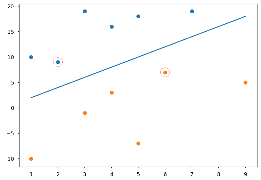
• Lets visualize the result

sv = clf.support_vectors_  # support vectors
w = clf.coef_[0]           # weights
b = clf.intercept_         # intercept

# w[0] * x + w[1] * y + b = 0
f = lambda x: -(b + w[0]*x) / w[1]

# plot training data
plt.scatter(*(zip(*X01)))
plt.scatter(*(zip(*X02)))

# plt decision boundary
plt.plot([1,9], [f(1), f(9)])

# mark support vectors
plt.scatter(*(zip(*sv)), zorder=1, facecolors='none', edgecolors='r', s=500);

Circle

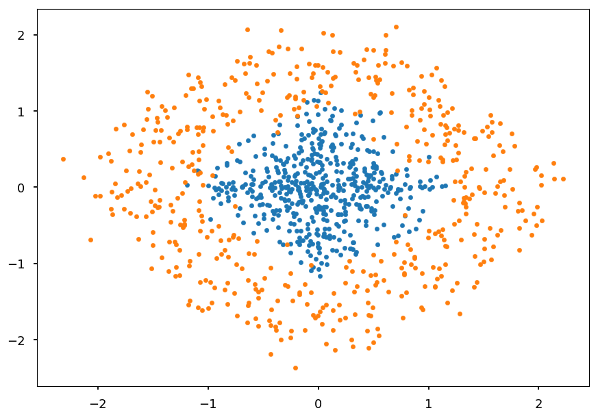
• For the simple non-linear problem lets consider once again points inside / outside a circle

• But this time let them also overlap a little bit die to some noise in data

def generate_circle_data(R1=0, R2=1, N=500):
  """Generate N points in a circle for radius range (R1, R2)"""
  r = lambda: R1 + np.random.random() * (R2 - R1) + np.random.normal(0, 0.2)

  return np.array([(r() * np.cos(ang), r() * np.sin(ang))
                   for ang in np.linspace(0, 2*np.pi, N)])

C01 = generate_circle_data()
C02 = generate_circle_data(1, 2)

plt.scatter(*C01.T, marker='.')
plt.scatter(*C02.T, marker='.');

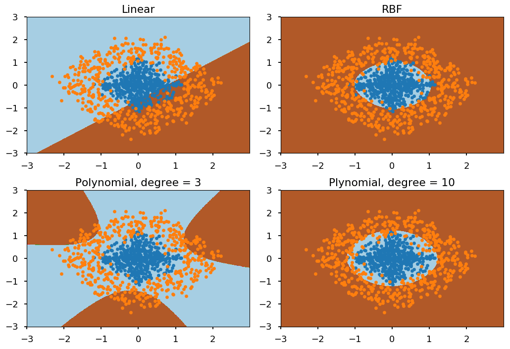
• We will consider 4 different kernels:

  • linear

  • polynomial of degree 3

  • polynomial of degree 10

  • Gaussian radial basis function (RBF)

# create classifier with different kernels
clf_linear = svm.SVC(kernel="linear")
clf_rbf = svm.SVC(kernel="rbf")
clf_poly3 = svm.SVC(kernel="poly", degree=3)
clf_poly10 = svm.SVC(kernel="poly", degree=10)

titles = ("Linear", "RBF", "Polynomial, degree = 3", "Plynomial, degree = 10")

# create a mesh to plot in
xx, yy = np.meshgrid(np.arange(-3, 3, 0.01), np.arange(-3, 3, 0.01))

# loop over classifiers
for i, clf in enumerate((clf_linear, clf_rbf, clf_poly3, clf_poly10)):
  # train classifier - assign -1 label for C01 and 1 for C02
  clf.fit(np.concatenate((C01, C02), axis=0), [-1]*len(C01) + [1]*len(C02))

  # visualize results
  plt.subplot(2, 2, i + 1)

  # decision boundary
  Z = clf.predict(np.c_[xx.ravel(), yy.ravel()])
  Z = Z.reshape(xx.shape)
  plt.contourf(xx, yy, Z, cmap=plt.cm.Paired)

  # training data
  plt.scatter(*C01.T, marker='.')
  plt.scatter(*C02.T, marker='.')

  plt.title(titles[i])

plt.tight_layout()

Multiclass classification

• There are two popular methods used to apply binary classificators to multiclass problem

• one-vs-rest (ovr) or one-vs-all (ova)

  • having $K$ classes with labels $y_i = \left\{1, \cdots, K\right\}$

  • train $K$ classifiers assuming $svm_i = 1$ and $svm_{j\neq i} = -1$

  • the prediction of a label for an unseen sample is based on a classifier which corresponds to the highest confidence score

• one-vs-one (ovo)

  • having $K$ classes with labels $y_i = \left\{1, \cdots, K\right\}$

  • train $K(K-1)/2$ classifiers for each possible pair of classes

  • the prediction is based on the voting scheme

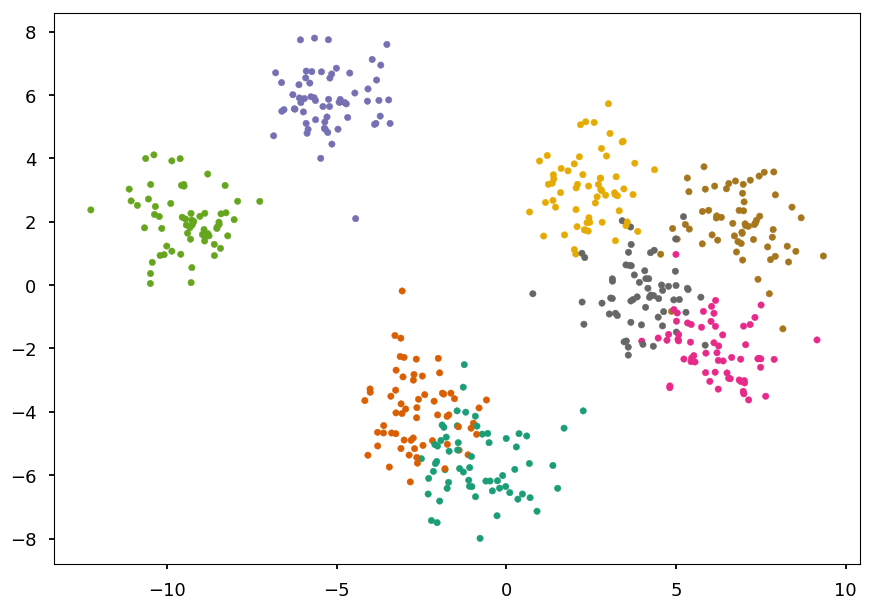
Example: blobs

• Lets use blobs form the previous lecture

from sklearn.datasets import make_blobs

# generate 5 blobs with fixed random generator
X, Y = make_blobs(n_samples=500, centers=8, random_state=300)

plt.scatter(*X.T, c=Y, marker='.', cmap='Dark2');

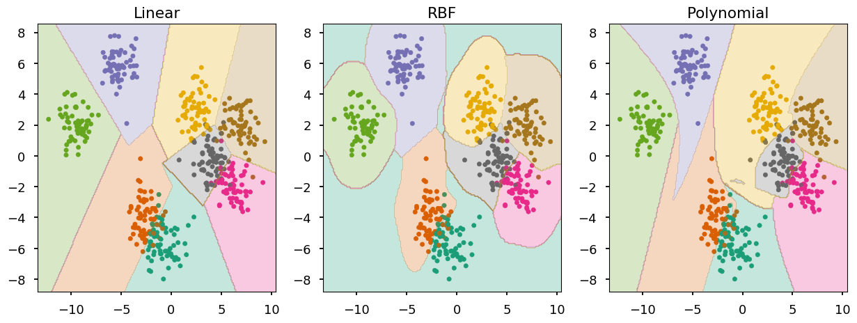
• We can use the same function as last time to train and visualize

def train_and_look(classifier, X, Y, ax=None, title='', cmap='Dark2'):
  """Train classifier on (X,Y). Plot data and prediction."""
  # create new axis if not provided
  ax = ax or plt.gca();

  ax.set_title(title)

  # plot training data
  ax.scatter(*X.T, c=Y, marker='.', cmap=cmap)

  # train a cliassifier
  classifier.fit(X, Y)

  # create a grid of testing points
  x_, y_ = np.meshgrid(np.linspace(*ax.get_xlim(), num=200),
                       np.linspace(*ax.get_ylim(), num=200))

  # convert to an array of 2D points
  test_data = np.vstack([x_.ravel(), y_.ravel()]).T

  # make a prediction and reshape to grid structure 
  z_ = classifier.predict(test_data).reshape(x_.shape)

  # arange z bins so class labels are in the middle
  z_levels = np.arange(len(np.unique(Y)) + 1) - 0.5

  # plot contours corresponding to classifier prediction
  ax.contourf(x_, y_, z_, alpha=0.25, cmap=cmap, levels=z_levels)

fig, ax = plt.subplots(1, 3, figsize=(15,5))

title = ("Linear", "RBF", "Polynomial")

settings = ({"kernel": "linear"}, {"kernel": "rbf"},
            {"kernel": "poly", "degree": 5})

# train and look at SVM with different kernels
for i in range(0, 3):
  train_and_look(svm.SVC(**settings[i]), X, Y,
                 ax=ax[i], title=title[i])

SVM regression

• Lets consider the problem of approximating the set of data $\left\{(\vec x_1, y_1), \cdots, (\vec x_N, y_N)\right\}$, where $\vec x_i \in \mathcal{R}^n$ and $y_i \in \mathcal{R}$ with a linear function:

  
  $f(\vec x) = \left<\vec w, \vec x\right> + b$

  
  

• In epsilon-insensitive SVM ($\varepsilon$-SVM) the goal is to find $f(x)$ that deviates from $y_i$ by a value not greater than $\varepsilon$ for each training point, and at the same time is as flat as possible.

• And once again we end up with a optimization problem:

  
  $\left.\begin{array}{cc}\text{minimize}_{w,b} & \frac{1}{2}|\vec w|^2 \\\text{subject to} & y_i - \left<\vec w, \vec x_i\right> - b \leq \varepsilon\\ & \left<\vec w, \vec x_i\right> + b - y_i \leq \varepsilon\end{array}\right.$

  
  

• It is enough if such $f$ actually exists

• However, analogously to soft margin, one can allow for some errors by introducing slack variables $\xi_i$ and $\xi^*_i$, and reformulate the optimization problem:

  
  $\left.\begin{array}{cc}\text{minimize}_{w,b} & \frac{1}{2}|\vec w|^2 + C\sum\limits_{i=1}^N(\xi_i + \xi^*_i) \\\text{subject to} & y_i - \left<\vec w, \vec x_i\right> - b \leq \varepsilon + \xi_i\\ & \left<\vec w, \vec x_i\right> + b - y_i \leq \varepsilon + \xi^*_i \\ & \xi_i, \xi^*_i \geq 0\end{array}\right.$

  
  

• The corresponding dual problem is given by:

  
  $\left.\begin{array}{cc}\text{minimize}_{\mu} & -\frac{1}{2}\sum\limits_{i, j = 1}^N(\mu_i - \mu^*_i)(\mu_j - \mu^*_j)\left<\vec x_i, \vec x_j\right> - \varepsilon\sum\limits_{i=1}^N(\mu_i + \mu^*_i) + \sum\limits_{i=1}^Ny_i(\mu_i - \mu^*_i)\\\text{subject to} & \sum\limits_{i=1}^N(\mu_i - \mu^*_i) = 0 \\ & \mu_i, \mu^*_i\in\left[0, C\right]\end{array}\right.$

  
  

• And the solution is given by: $\vec w = \sum\limits_{i=1}^N(\mu_i - \mu^*_i)\vec x_i$, thus:

  
  $f(\vec x) = \sum\limits_{i=1}^N(\mu_i - \mu^*_i)\left<\vec x_i, \vec x\right> + b$

  
  

• Or for the kernelized version:

  
  $f(\vec x) = \sum\limits_{i=1}^N(\mu_i - \mu^*_i)K(\vec x_i, \vec x)+ b$

  
  

• The intercept $b$ can be calculate for any support vector as $f(\vec x_{SV}) = y_{SV}$

Example - Boston Housing dataset

from sklearn.datasets import load_boston

boston = load_boston()

print(boston.DESCR)

Boston House Prices dataset
===========================

Notes
------
Data Set Characteristics:

    :Number of Instances: 506

    :Number of Attributes: 13 numeric/categorical predictive

    :Median Value (attribute 14) is usually the target

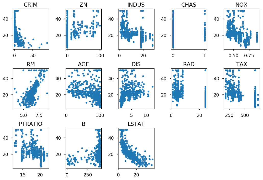
    :Attribute Information (in order):
        - CRIM     per capita crime rate by town
        - ZN       proportion of residential land zoned for lots over 25,000 sq.ft.
        - INDUS    proportion of non-retail business acres per town
        - CHAS     Charles River dummy variable (= 1 if tract bounds river; 0 otherwise)
        - NOX      nitric oxides concentration (parts per 10 million)
        - RM       average number of rooms per dwelling
        - AGE      proportion of owner-occupied units built prior to 1940
        - DIS      weighted distances to five Boston employment centres
        - RAD      index of accessibility to radial highways
        - TAX      full-value property-tax rate per $10,000
        - PTRATIO  pupil-teacher ratio by town
        - B        1000(Bk - 0.63)^2 where Bk is the proportion of blacks by town
        - LSTAT    % lower status of the population
        - MEDV     Median value of owner-occupied homes in $1000's

    :Missing Attribute Values: None

    :Creator: Harrison, D. and Rubinfeld, D.L.

This is a copy of UCI ML housing dataset.
http://archive.ics.uci.edu/ml/datasets/Housing


This dataset was taken from the StatLib library which is maintained at Carnegie Mellon University.

The Boston house-price data of Harrison, D. and Rubinfeld, D.L. 'Hedonic
prices and the demand for clean air', J. Environ. Economics & Management,
vol.5, 81-102, 1978.   Used in Belsley, Kuh & Welsch, 'Regression diagnostics
...', Wiley, 1980.   N.B. Various transformations are used in the table on
pages 244-261 of the latter.

The Boston house-price data has been used in many machine learning papers that address regression
problems.

**References**

   - Belsley, Kuh & Welsch, 'Regression diagnostics: Identifying Influential Data and Sources of Collinearity', Wiley, 1980. 244-261.
   - Quinlan,R. (1993). Combining Instance-Based and Model-Based Learning. In Proceedings on the Tenth International Conference of Machine Learning, 236-243, University of Massachusetts, Amherst. Morgan Kaufmann.
   - many more! (see http://archive.ics.uci.edu/ml/datasets/Housing)

Visualize dataset

for i, feature in enumerate(boston.data.T):
  plt.subplot(3, 5, i+1)
  plt.scatter(feature, boston.target, marker='.')
  plt.title(boston.feature_names[i])

plt.tight_layout()

import pandas as pd

boston_pd = pd.DataFrame(boston.data)     # load features
boston_pd.columns = boston.feature_names  # add features names
boston_pd['PRICE'] = boston.target        # add a column with price

boston_pd.head()

	CRIM	ZN	INDUS	CHAS	NOX	RM	AGE	DIS	RAD	TAX	PTRATIO	B	LSTAT	PRICE
0	0.00632	18.0	2.31	0.0	0.538	6.575	65.2	4.0900	1.0	296.0	15.3	396.90	4.98	24.0
1	0.02731	0.0	7.07	0.0	0.469	6.421	78.9	4.9671	2.0	242.0	17.8	396.90	9.14	21.6
2	0.02729	0.0	7.07	0.0	0.469	7.185	61.1	4.9671	2.0	242.0	17.8	392.83	4.03	34.7
3	0.03237	0.0	2.18	0.0	0.458	6.998	45.8	6.0622	3.0	222.0	18.7	394.63	2.94	33.4
4	0.06905	0.0	2.18	0.0	0.458	7.147	54.2	6.0622	3.0	222.0	18.7	396.90	5.33	36.2

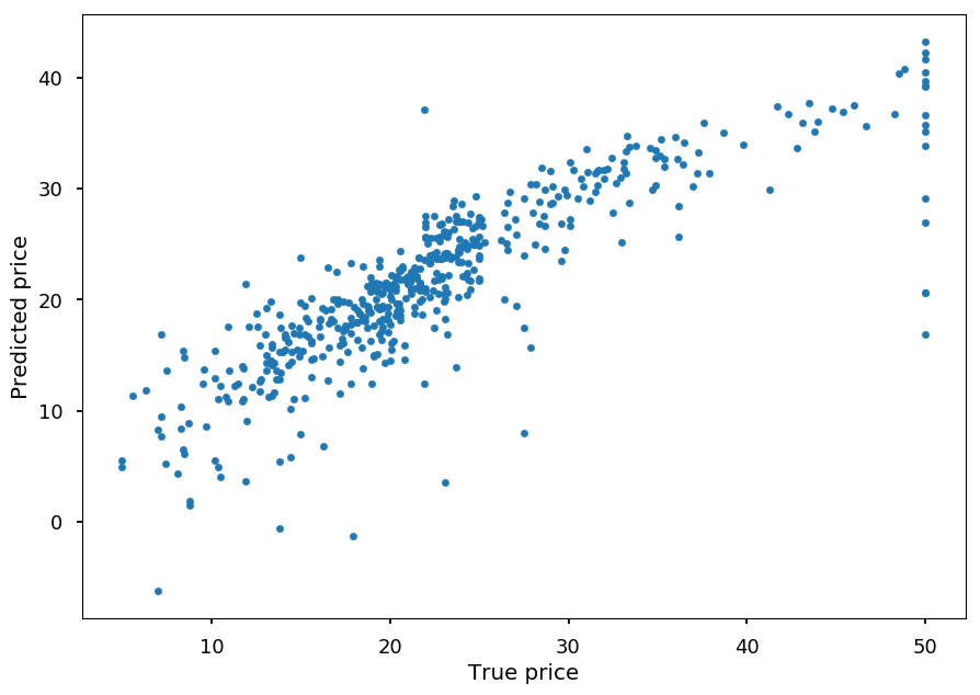
Test SVR

• Below there is a result for the linear kernel - feel free to play with kernels and/or parameter $C$ on your own

from sklearn.svm import SVR

regressor = SVR(kernel="linear")
regressor.fit(boston.data, boston.target)

prediction = regressor.predict(boston.data)

plt.xlabel("True price")
plt.ylabel("Predicted price")

plt.scatter(boston.target, prediction, marker='.');

Summary

• Support vector machine is a powerful model for both classification and regression

• It guarantees finding the optimal hyperplane / decision boundary (if exists)

• It is effective with high dimensional data

• The dual formulation of the optimization problem allows easily to introduce kernels and deal with non-linear data

• It has just few hyperparameters: kernel + kernel's parameters and $C$

• Inference is fast as it depends only on a subset of training samples (support vectors) - although training may be slow for large datasets