

Decision Trees¶

Graphviz¶

Installing graphviz¶

!apt install -y graphviz
!pip install graphviz

A tree example¶

from graphviz import Digraph

styles = {
    'top': {'shape': 'ellipse', 'style': 'filled', 'color': 'lightblue'},
    'no':  {'shape': 'circle', 'style': 'filled', 'color': 'red'},
    'yes': {'shape': 'circle', 'style': 'filled', 'color': 'lightgreen'},
    'qst': {'shape': 'rect'}
}

example_tree = Digraph()

example_tree.node('top', 'Should I attend the ML lecture?', styles['top'])
example_tree.node('q1', 'Do I fulfill requirements?', styles['qst'])

example_tree.node('q2', 'Do I like CS?', styles['qst'])
example_tree.node('no1', 'No ', styles['no'])

example_tree.node('q3', 'Is the lecture early in the morning?', styles['qst'])
example_tree.node('no2', 'No ', styles['no'])

example_tree.node('no3', 'No ', styles['no'])
example_tree.node('yes', 'Yes', styles['yes'])

example_tree.edge('top', 'q1')

example_tree.edge('q1', 'q2', 'Yes')
example_tree.edge('q1', 'no1', 'No')

example_tree.edge('q2', 'q3', 'Yes')
example_tree.edge('q2', 'no2', 'No')

example_tree.edge('q3', 'no3', 'Yes')
example_tree.edge('q3', 'yes', 'No')

example_tree

svg

Introduction¶

Decision trees¶

Supervised learning algorithm - training dataset with known labels
Eager learning - final model does not need training data to make prediction (all parameters are evaluated during learning step)
It can do both classification and regression
A decision tree is built from:
- decision nodes - correspond to features (attributes)
- leaf nodes - correspond to class labels
The root of a tree is (should be) the best predictor (feature)

Example¶

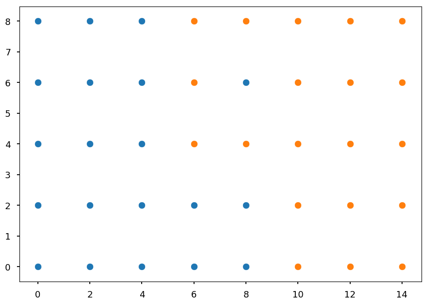
import matplotlib.pyplot as plt
import numpy as np

# just to overwrite default colab style
plt.style.use('default')
plt.style.use('seaborn-talk')

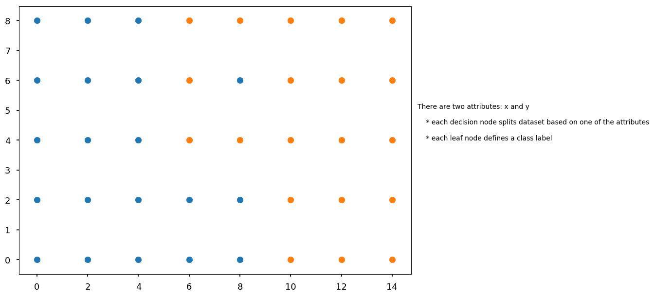
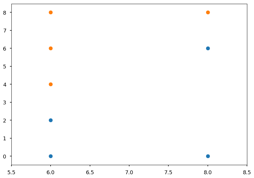
# first define some points representing two classes
grid = np.mgrid[0:10:2, 0:10:2]
set01 = np.vstack([grid[0].ravel(), grid[1].ravel()]).T
set01 = np.delete(set01, [17, 18, 19, 22, 24], axis=0)

grid = np.mgrid[6:16:2, 0:10:2]
set02 = np.vstack([grid[0].ravel(), grid[1].ravel()]).T
set02 = np.delete(set02, [0, 1, 5, 6, 8], axis=0)

plt.scatter(*set01.T)
plt.scatter(*set02.T)

plt.text(15, 4, "There are two attributes: x and y\n\n"
                "    * each decision node splits dataset based on one of the attributes\n\n"
                "    * each leaf node defines a class label");

png

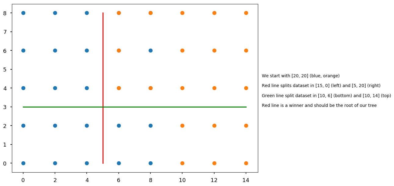
plt.scatter(*set01.T)
plt.scatter(*set02.T)

plt.plot([5, 5], [0, 8], 'r')
plt.plot([0, 14], [3, 3], 'g')

plt.text(15, 3, "We start with [20, 20] (blue, orange)\n\n"
                "Red line splits dataset in [15, 0] (left) and [5, 20] (right)\n\n"
                "Green line split dataset in [10, 6] (bottom) and [10, 14] (top)\n\n"
                "Red line is a winner and should be the root of our tree");

png

tree = Digraph()

tree.edge("x > 5?\n[20, 20]", "blue\n[15, 0]", "No")
tree.edge("x > 5?\n[20, 20]", "y > 3?\n[5, 20]", "Yes")

tree.edge("y > 3?\n[5, 20]", "x > 9?\n[4, 6]", "No")
tree.edge("y > 3?\n[5, 20]", "almost orange\n[1, 14]", "Yes")

tree.edge("x > 9?\n[4, 6]", "blue\n[4, 0]", "No")
tree.edge("x > 9?\n[4, 6]", "orange\n[0, 6]", "Yes")

tree.edge("almost orange\n[1, 14]", "Should we continue?\nOr would it be overfitting?")

tree

svg

It is important to start with good predictor
- Our choice of the root classifies 37.5% of points in the first step
- Note, that we could also start with x > 9?
- However, if we started with y > 3 we would never classify a point in the first step - does it mean that it is worse choice?

tree = Digraph()

tree.edge("y > 3?\n[20, 20]", "x > 9?\n[10, 6]", "No")
tree.edge("y > 3?\n[20, 20]", "x > 5?\n[10, 14]", "Yes")

tree.edge("x > 9?\n[10, 6]", "blue\n[10, 0]", "No")
tree.edge("x > 9?\n[10, 6]", "orange\n[0, 6]", "Yes")

tree.edge("x > 5?\n[10, 14]", "blue\n[9, 0]", "No")
tree.edge("x > 5?\n[10, 14]", "almost orange\n[1, 14]", "Yes")

tree

svg

In this case we never have to make more than 2 checks
There are two open questions to answer:
- How to automate the procees of chosing nodes?
- How deep should we go?

ID3 and C4.5 algorithms¶

We start with algorithms based on information theory
- ID3 (Iterative Dichotomiser 3)
- C4.5 - extension of ID3 (why C4.5? C stands for programming language and 4.5 for version?)
- C5.0/See5 - improved C4.5 (commercial; single-threaded Linux version is available under GPL though)
The idea is to find nodes which maximize information gain

Information gain¶

Self-information¶

Let $X = (x_1, x_2, ..., x_n)$ be our information source (feature), e.g. weather condition: $x_1$ = sunny, $x_2$ = overcast, $x_3$ = rainy
And let $P = (p_1, p_2, ..., p_n)$ be corresponding probrability distribution (or more precisely - probability mass function)
We want some measure of information $I$ provided by an event. It should satisfy the following properties:
- $I$ depends only on the probability of $x_i$ , thus $I \equiv I(p_i)$
- $I$ is continuous and deacreasing function of $p_i$
- $I$ is non-negative and $I(1) = 0$
- if $p_i = p_{i, 1} \cdot p_{i, 2}$ (independent events) then $I(p_i) = I(p_{i, 1}) + I(p_{i, 2})$
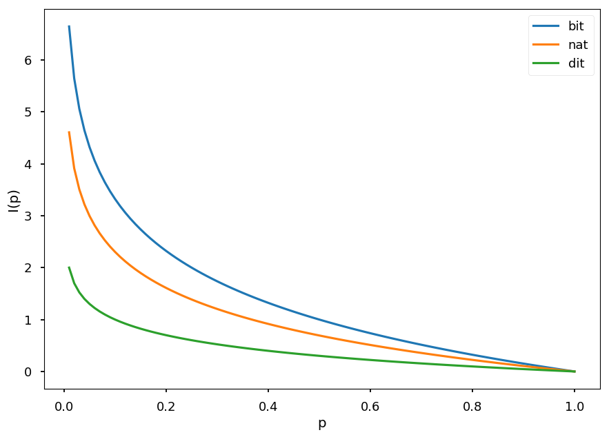
Logarithmic function satisfies all above condition, so we define self-information as:

$I(p) = -\log(p)$
- The most common log base is 2 and then information is in shannons (Sh), also known as bits
- In the case of natural logarithm the unit is nat (natural unit of information)
- In the case of base 10 the unit is hartley (Hart), also known as dit

x = np.arange(0.01, 1.01, 0.01)

plt.xlabel("p")
plt.ylabel("I(p)")

plt.plot(x, -np.log2(x), label="bit")
plt.plot(x, -np.log(x), label="nat")
plt.plot(x, -np.log10(x), label="dit")

plt.legend();

png

Lets X = (head, tail) with P = (0.5, 0.5)
- We get 1 Sh of information
Lets X = (sunny, overcast, rainy) with P = (0.25, 0.75, 0.25)
- If it is overcast, we get 0.415 Sh of information
- Otherwise, we get 2 Sh of information
If an event is more likely we learn less

Information entropy¶

Also called Shannon entropy (after the father of intromation theory)
Usually information entropy is denoted as $H$
$H$ is defined as the weighted average of the self-information of all possible outcomes

$H(X) = \sum\limits_{i=1}^N p_i \cdot I(p_i) = -\sum\limits_{i=1}^N p_i\cdot\log(p_i)$
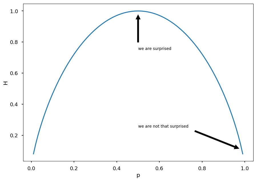
Lets consider two case scenario with $P = (p, 1 - p)$ , so entropy is given by $H = -p \log(p) - (1 - p) \log(1 - p)$

p = np.arange(0.01, 1.0, 0.01)

plt.xlabel("p")
plt.ylabel("H")

plt.annotate('we are surprised', xy=(0.5, 1), xytext=(0.5, 0.75),
             arrowprops=dict(facecolor='black', shrink=0.1))

plt.annotate('we are not that surprised', xy=(1, 0.1), xytext=(0.5, 0.25),
             arrowprops=dict(facecolor='black', shrink=0.1))

plt.plot(p, -p * np.log2(p) - (1 - p) * np.log2(1 - p));

png

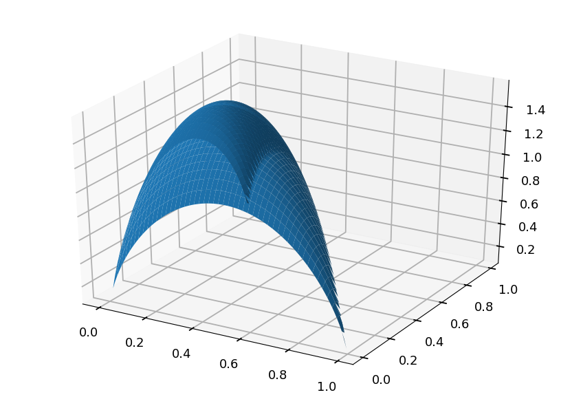
Lets consider three case scenario with $P = (p, q, 1 - p - q)$ , so entropy is given by $H = -p \log(p) - q\log(q) - (1 - p - q) \log(1 - p - q)$

from mpl_toolkits import mplot3d

# grid of p, q probabilities
p, q = np.meshgrid(np.arange(0.01, 1.0, 0.01), np.arange(0.01, 1.0, 0.01))

# remove (set to 0) points which do not fulfill P <= 1
idx = p + q > 1
p[idx] = 0
q[idx] = 0

# calculate entropy (disable warnings - we are aware of log(0))
np.warnings.filterwarnings('ignore')
h = -p * np.log2(p) - q * np.log2(q) - (1 - p - q) * np.log2(1 - p - q)

# make a plot
plt.axes(projection='3d').plot_surface(p, q, h);

png

Information gain¶

Let $T$ be the set of training samples with $n$ possible outcomes, thus $T = \{T_1, T_2, ..., T_n\}$
The entropy is given by

$H(T) = -\sum\limits_{i=1}^N p_i\cdot\log(p_i) = -\sum\limits_{i=1}^N \frac{|T_i|}{|T|}\cdot\log(\frac{|T_i|}{|T|})$
We can also calulate the entropy after $T$ was partitioned in $T_i$ with respect to some feature $X$

$H(T, X) = \sum\limits_{i=1}^N p_i\cdot H(T_i)$
And the information gain is defined as

$G(X) = H(T) - H(T, X)$

Example¶

Lets calculate some example step by step
Lets consider a fake dataset
- two classes: C01, C02
- three features: X1, X2, X3

   X1  ||  A  |  A  |  A  |  B  |  B  |  C  |  C  |  C  |  C  |
---------------------------------------------------------------
   X2  ||  0  |  0  |  1  |  1  |  0  |  1  |  1  |  1  |  0  |
---------------------------------------------------------------
   X3  || RED | GRN | GRN | BLU | RED | GRN | BLU | RED | GRN |
===============================================================
 Class || C01 | C01 | C02 | C02 | C02 | C02 | C01 | C01 | C02 |

from math import log

def entropy(*probs):
  """Calculate information entropy"""
  try:
    total = sum(probs)
    return sum([-p / total * log(p / total, 2) for p in probs])
  except:
    return 0

print(entropy(4, 5), entropy(2, 1), entropy(2, 2))

0.9910760598382222 0.9182958340544896 1.0

The root entropy
- We have 9 samples: 4 belong to class C01 and 5 to C02
  
  $H(T) = -\frac{4}{9}\log(\frac{4}{9}) - \frac{5}{9}\log(\frac{5}{9}) = 0.99$
Now lets consider feature X1, which splits data into subsets $T_1$ , $T_2$ , and $T_3$ (with X1 value A, B, and C, respectively)
- Within $T_1$ there are 3 samples: 2 from C01 and 1 from C02
  
  $H(T_1) = -\frac{2}{3}\log(\frac{2}{3}) - \frac{1}{3}\log(\frac{1}{3}) = 0.92$
- Within $T_2$ there are 2 samples: 0 from C01 and 2 from C02
  
  $H(T_2) = -\frac{2}{2}\log(\frac{2}{2}) - \frac{0}{2}\log(\frac{0}{2}) = 0.00$
- Within $T_3$ there are 4 samples: 2 from C01 and 2 from C02
  
  $H(T_3) = -\frac{2}{4}\log(\frac{2}{4}) - \frac{2}{4}\log(\frac{2}{4}) = 1.00$
- The resulting entropy is
  
  $H(T, X1) = \frac{3}{9}\cdot H(T_1) + \frac{2}{9}\cdot H(T_2) + \frac{4}{9}\cdot H(T_3) = 0.75$
- Thus, infromation gain if the set is split according to X1
  
  $G(X1) = H(T) - H(T, X1) = 0.99 - 0.75 = 0.24 \mbox{ Sh }$

ID3 algorithm¶

For every attribute (feature) calculate the entropy
Split the training set using the one for which information gain is maximum
Continue recursively on subsets using remaining features

Play Golf dataset¶

Popular dataset to explain decision trees
4 features:
- outlook: rainy, overcast, sunny
- temperature: cool, mild, hot
- humidity: normal, high
- windy: false, true
Possible outcomes (play golf?):
- false
- true

import pandas as pd

# first row = headers
src = "http://chem-eng.utoronto.ca/~datamining/dmc/datasets/weather_nominal.csv"

golf_data = pd.read_csv(src)

golf_data

	Outlook	Temperature	Humidity	Windy	Play golf
0	Rainy	Hot	High	False	No
1	Rainy	Hot	High	True	No
2	Overcast	Hot	High	False	Yes
3	Sunny	Mild	High	False	Yes
4	Sunny	Cool	Normal	False	Yes
5	Sunny	Cool	Normal	True	No
6	Overcast	Cool	Normal	True	Yes
7	Rainy	Mild	High	False	No
8	Rainy	Cool	Normal	False	Yes
9	Sunny	Mild	Normal	False	Yes
10	Rainy	Mild	Normal	True	Yes
11	Overcast	Mild	High	True	Yes
12	Overcast	Hot	Normal	False	Yes
13	Sunny	Mild	High	True	No

Play golf entropy¶

entropy(9, 5)

0.9402859586706309

| Play golf |
=============
| yes | no  |  -> H(T) = 0.94
-------------
|  9  |  5  |

Play golf vs outlook¶

                   | Play golf |
                   =============
                   | yes | no  |
        ------------------------
        | sunny    |  3  |  2  |  5
outlook | overcast |  4  |  0  |  4
        | rainy    |  2  |  3  |  5
        ------------------------
                      9     5

entropy(3, 2), 0, entropy(2, 3)

(0.9709505944546686, 0, 0.9709505944546686)

\begin{eqnarray} H(\mbox{sunny}) & = & 0.97 \\ H(\mbox{rainy}) & = & 0.97 \\ H(\mbox{overcast}) & = & 0 \end{eqnarray}

\begin{eqnarray} H(T, \mbox{outlook}) & = & P(\mbox{sunny})\cdot H(\mbox{sunny}) + P(\mbox{overcast})\cdot H(\mbox{overcast}) + P(\mbox{rainy})\cdot H(\mbox{rainy}) \\ & = & \frac{5}{14}\cdot 0.97 + \frac{4}{14} \cdot 0 + \frac{5}{14}\cdot 0.97 = 0.69 \end{eqnarray}

\begin{eqnarray} G(\mbox{outlook}) & = & H(T) - H(T, \mbox{outlook}) = 0.94 - 0.69 = 0.25 \end{eqnarray}

Results for all features¶

                    | Play golf |                         | Play golf |
                    =============                         =============
                    | yes | no  |                         | yes | no  |
         ------------------------                 --------------------
         | sunny    |  3  |  2  |                 | hot   |  2  |  2  |
 outlook | overcast |  4  |  0  |     temperature | mild  |  4  |  2  |
         | rainy    |  2  |  3  |                 | cool  |  3  |  1  |
         ------------------------                 --------------------
            Info. gain = 0.25                       Info gain = 0.03


                    | Play golf |                         | Play golf |
                    =============                         =============
                    | yes | no  |                         | yes | no  |
         ------------------------                 --------------------
         | high     |  3  |  4  |                 | false |  6  |  2  |
humidity | normal   |  6  |  1  |           windy | true  |  3  |  3  |
         ------------------------                 --------------------
            Info. gain = 0.15                       Info gain = 0.05

Root of the tree¶

Start building a tree with the feature with the largest information gain: outlook
A branch with entropy 0 is a leaf node: overcast
Other branches must be spliited using other features

tree = Digraph()

tree.edge("outlook", "sunny")
tree.edge("outlook", "overcast")
tree.edge("outlook", "rainy")

tree.edge("overcast", "yes")

tree

svg

Next branch¶

golf_data.loc[golf_data['Outlook'] == "Sunny"]

	Outlook	Temperature	Humidity	Windy	Play golf
3	Sunny	Mild	High	False	Yes
4	Sunny	Cool	Normal	False	Yes
5	Sunny	Cool	Normal	True	No
9	Sunny	Mild	Normal	False	Yes
13	Sunny	Mild	High	True	No

In general, one should calculate information gain for each feature for this subset
In this case it is clear that we can take windy

tree.edge("sunny", "windy")

tree.edge("windy", "false")
tree.edge("windy", "true")

tree.edge("false", "yes")
tree.edge("true", "no")

tree

svg

Last branch¶

golf_data.loc[golf_data['Outlook'] == "Rainy"]

	Outlook	Temperature	Humidity	Windy	Play golf
0	Rainy	Hot	High	False	No
1	Rainy	Hot	High	True	No
7	Rainy	Mild	High	False	No
8	Rainy	Cool	Normal	False	Yes
10	Rainy	Mild	Normal	True	Yes

tree.edge("rainy", "humidity")

tree.edge("humidity", "high")
tree.edge("humidity", "normal")

tree.edge("normal", "yes")
tree.edge("high", "no ")

tree

svg

Summary¶

We got the final tree for Play Golf dataset using ID3 algorithm
We do not even use temperature attribute (for which information gain was 0.03)
The main problem is that the algorithm may overfit easily (tree does not stop growing until the whole training set is classified)
- Imagine some crazy guys went playing on a rainy, windy day with high humidity, beacaue it was still hot
- With this extra data point we would have to create more branches
- Is one unique data sample worth to extend the whole tree?
And there is more disadvantages:
- It handles only discrete attributes
- There is a strong bias for features with many possible outcomes
- And finally, it does not handle missing values

C4.5 algorithm¶

C4.5 introduces some improvements to ID3:
- continuous values using threshold
- tree pruning to avoid overfitting
- normalized information gain
- missing values

Information gain ratio¶

To avoid a bias in favor of features with a lot of different values C4.5 uses information gain ratio instead of information gain
Lets define intrinsic value $V$ of an attribute $X$ as
$V(X) = -\sum\limits_{i=1}^N \frac{|T_i|}{|T|}\cdot\log(\frac{|T_i|}{|T|})$
where $T_i$ are samples corresponding to $i$ -th possible value of $X$ feature
Information gain ratio $R(X)$ is defined as
$R(X) = \frac{G(X)}{V(X)}$

Example¶

Lets consider a fake data set
The goal is to determine if someone plays or not video games
We have three features:
- name - mostly unique
- sex - 50% females and 50% males
- age - just old or young
Looking at data we can say that
- most young people play video games, why old people don't
- sex does not matter
- names are almost distinct

     name   ||  John  |  Mark  |  Anne  |  Adam  |  John  |  Alex  |  Alex  |  Xena  |  Tina  |  Lucy  |
--------------------------------------------------------------------------------------------------------
     sex    ||   M    |   M    |   F    |   M    |   M    |   F    |   M    |   F    |   F    |   F    |
--------------------------------------------------------------------------------------------------------
     age    ||  old   | young  |  old   | young  | young  | young  |  old   |  old   | young  | young  |
========================================================================================================
 play games ||   N    |   Y    |   Y    |   Y    |   Y    |   N    |   N    |   N    |   Y    |   Y    |

Information gain for name

h = entropy(4, 6)  # dataset entropy H(T)

# one John plays and the other one doesn't
# in other cases entropy = 0
g_name = h - 2/10 * entropy(1, 1)

print(g_name)

0.7709505944546686

Information gain for sex

# 5 men - 3 play
# 5 women - 3 play
g_sex = h - 5/10 * entropy(2, 3) - 5/10 * entropy(2, 3)

print(g_sex)

0.0

Information gain for age

# 4 old people - 1 plays
# 6 young people - 5 play
g_age = h - 4/10 * entropy(1, 3) - 6/10 * entropy(1, 5)

print(g_age)

0.256425891682003

In ID3 a feature with entropy = 0 is always a winner
- Imagine having all distinct values (e.g. credit card numbers)
In this case we would choose name as the best predictor
- Creating a tree with 8 branches (from 10 samples)
- Training data would be perfectly classify
- But it is unlikely that the algorithm would be able to generalize for unseen data
Lets calculate information gain ratio and see how it changes the choice of the best feature
Information gain ratio for name

# 2x John, 2x Alex, 6x unique name 
g_name / entropy(2, 2, *[1]*6)

0.26384995435159336

Information gain ratio for sex

# 5 males and 5 females - zero stays zero though
g_sex / entropy(5, 5)

0.0

Information gain ratio for age

# 4x old and 6x young
g_age / entropy(4, 6)

0.26409777505314147

Based on information gain ratio we choose age as the best predictor
Because the denominator in a ratio penalizes features with many values

print("Two possible values:\n")

for i in range(0, 11):
  print("\t({}, {}) split -> entropy = {}".format(i, 10-i, entropy(i, 10-i)))

print("\n10 possible values:", entropy(*[1]*10))

Two possible values:

    (0, 10) split -> entropy = 0
    (1, 9) split -> entropy = 0.4689955935892812
    (2, 8) split -> entropy = 0.7219280948873623
    (3, 7) split -> entropy = 0.8812908992306927
    (4, 6) split -> entropy = 0.9709505944546686
    (5, 5) split -> entropy = 1.0
    (6, 4) split -> entropy = 0.9709505944546686
    (7, 3) split -> entropy = 0.8812908992306927
    (8, 2) split -> entropy = 0.7219280948873623
    (9, 1) split -> entropy = 0.4689955935892812
    (10, 0) split -> entropy = 0

10 possible values: 3.321928094887362

This datset was handcrafted to make a point, but I hope the message is still clear

Continuous values¶

Attributes with continuous values must be first discretize
The best way is to find an optimal threshold which splits the set
The optimal threshold is the one which maximize the infromation gain

Example¶

Lets consider the same example as before
But this time age has numerical values

     name   ||  John  |  Mark  |  Anne  |  Adam  |  John  |  Alex  |  Alex  |  Xena  |  Tina  |  Lucy  |
--------------------------------------------------------------------------------------------------------
     sex    ||   M    |   M    |   F    |   M    |   M    |   F    |   M    |   F    |   F    |   F    |
--------------------------------------------------------------------------------------------------------
     age    ||   50   |   18   |   65   |   24   |   31   |   18   |   50   |   50   |   24   |   31   |
========================================================================================================
 play games ||   N    |   Y    |   Y    |   Y    |   Y    |   N    |   N    |   N    |   Y    |   Y    |

The possible thesholds are therefore $\{18, 24, 31, 50\}$

# calculate entropy for all possible thresholds
e18 = 2/10 * entropy(1, 1) + 8/10 * entropy(3, 5)
e24 = 4/10 * entropy(1, 3) + 6/10 * entropy(3, 3)
e31 = 6/10 * entropy(1, 5) + 4/10 * entropy(3, 1)
e50 = 9/10 * entropy(4, 5) + 1/10 * entropy(0, 1)

print("With threshold = {}, entropy = {}".format(18, e18))
print("With threshold = {}, entropy = {}".format(24, e24))
print("With threshold = {}, entropy = {}".format(31, e31))
print("With threshold = {}, entropy = {}".format(50, e50))

With threshold = 18, entropy = 0.963547202339972
With threshold = 24, entropy = 0.9245112497836532
With threshold = 31, entropy = 0.7145247027726656
With threshold = 50, entropy = 0.8919684538544

The best test is if age > 31
- it splits the dataset to 6 samples (with 5 players) and 4 samples (with 3 non-players)
Please note, that the best threshold may change once a node is created

Unknown parameters¶

In the case some samples are incomplete one needs to correct the information gain
The information gain is calculated as before for samples with known attributes
But then it is normalized with respect to the probability that the given attribute has known values
Lets define the factor $F$ as the ratio of the number of samples with known value for a given feature to the number of all samples in a dataset
Then information gain is defines as
$G(X) = F\cdot (H(T) - H(T, X))$
Please note, that $F = 1$ if all values are known
Otherwise, information gain is scaled accordingly

Pruning¶

The algorithm creates as many nodes as needed to classify all test samples
It may lead to overfitting and the resulting tree would fail to classify correctly unseen samples
To avoid this one can prune a tree
- pre-pruning (early stopping)
  - stop building a tree before leaves with few samples are produced
  - how to decide when it is good time to stop? e.g. using cross-validation on validation set (stop if the error does not increase significantly)
  - underfitting if stop to early
- post-pruning
  - let a tree grow completely
  - then go from bottom to top and try to replace a node with a leaf
  - if there is improvement in accuracy - cut a tree
  - if the accuracy stays the same - cut a tree (Occam's razor)
  - otherwise leave a node

First example - step by step¶

Lets consider the problem from the beginning of the lecture
Our dataset has 20 blue points and 20 orange points
Each point has two features (both are numerical)
We expect overfitting if pruning is not applied
We will calculate everything step by step (it is boring, but demonstrates how the algorithm works)

# first define some points representing two classes
grid = np.mgrid[0:10:2, 0:10:2]
set01 = np.vstack([grid[0].ravel(), grid[1].ravel()]).T
set01 = np.delete(set01, [17, 18, 19, 22, 24], axis=0)

grid = np.mgrid[6:16:2, 0:10:2]
set02 = np.vstack([grid[0].ravel(), grid[1].ravel()]).T
set02 = np.delete(set02, [0, 1, 5, 6, 8], axis=0)

plt.scatter(*set01.T)
plt.scatter(*set02.T);

png

Validation set¶

We will use 10 points from the dataset for validation
This time selected manually to perform by hand calculations
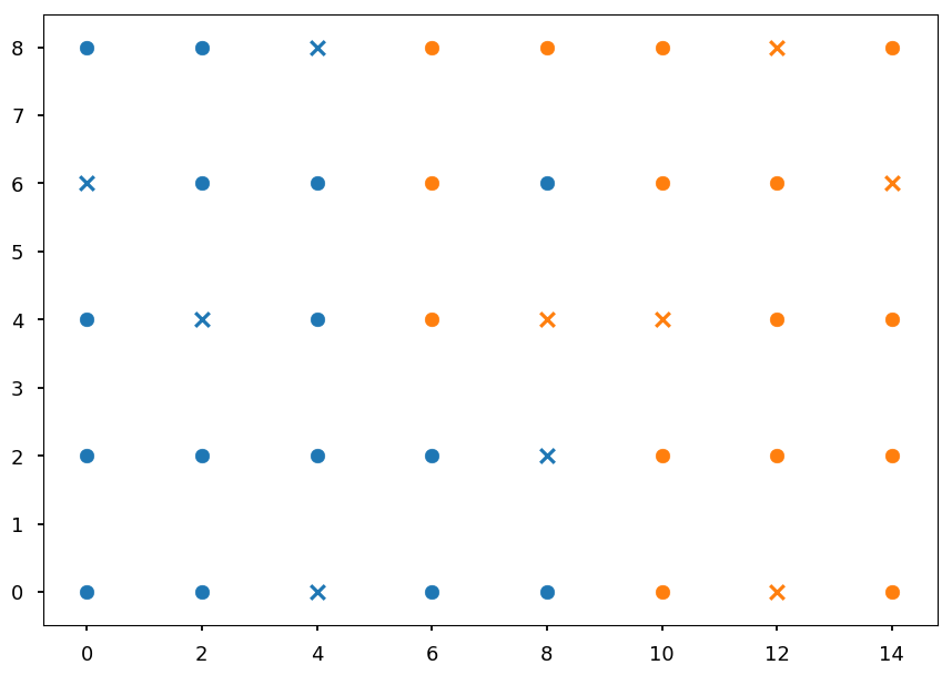
On the plot below X denotes validation samples

# split dataset to training and validation set
# note, we should splt them randomly
# but here we do this by hand
valid_idx = [3, 7, 10, 14, 18]

blue_valid = set01[valid_idx]
blue_train = np.delete(set01, valid_idx, axis=0)

orange_valid = set02[valid_idx]
orange_train = np.delete(set02, valid_idx, axis=0)

# circles - training set
# x - validation set
plt.scatter(*blue_train.T)
plt.scatter(*blue_valid.T, color='C0', marker='x')
plt.scatter(*orange_train.T)
plt.scatter(*orange_valid.T, color='C1', marker='x');

png

Thresholds finder¶

When building a tree we need to calculate information gain for every threshold in current subset
Every subset $S$ has $N_b$ blue samples and $N_o$ orange samples
After split into accoring to some threshold we get two subsets
- $n_b$ of blue points and $n_o$ of orange points ( $S_1$ )
- $N_b - n_b$ of blue points and $N_o - n_o$ of orange points ( $S_2$ )

def info_gain(Nb, No, nb, no):
  """Calculate information gain for given split"""
  h = entropy(Nb, No) # H(S)
  total = Nb + No     # total number of samples
  subtotal = nb + no  # number of samples in subset

  return h - subtotal / total * entropy(nb, no) \
           - (total - subtotal) / total * entropy(Nb - nb, No - no)

Feature X¶

We need to calculate information gain ratio for the best threshold (the one that maximize information gain)
Possible thresholds $\{0, 2, 4, 6, 8, 10, 12\}$

Nb = 15
No = 15

splits = {"0": (4, 0), "2 ": (8, 0), "4": (11, 0), "6": (13, 3),
          "8": (15, 4), "10": (15, 8), "12": (15, 11)}

for threshold, (no, nb) in splits.items():
  print("Threshold = {}\t -> {}".format(threshold, info_gain(Nb, No, no, nb)))

Threshold = 0    -> 0.14818913558232172
Threshold = 2    -> 0.33824492595034883
Threshold = 4    -> 0.5297578726233217
Threshold = 6    -> 0.3525728312615027
Threshold = 8    -> 0.5297578726233217
Threshold = 10   -> 0.28538113149388267
Threshold = 12   -> 0.14818913558232172

We got the same cuts as predicted at the beginning of the lecture: $x > 4$ or $x > 8$
Lets choose $x > 4$ and calculate information gain ratio

# 4 samples with x = 0, 4 samples with x = 2 etc
info_gain(Nb, No, *splits["4"]) / entropy(4, 4, 3, 5, 3, 4, 3, 4)

0.1779055922617179

Feature Y¶

Repeat the procedure
This time possible thresholds = $\{0, 2, 4, 6\}$

Nb = 15
No = 15

splits = {"0": (4, 2), "2": (8, 5), "4": (10, 8), "6": (13, 11)}

for threshold, (no, nb) in splits.items():
  print("Threshold = {}\t -> {}".format(threshold, info_gain(Nb, No, no, nb)))

Threshold = 0    -> 0.02035297064032593
Threshold = 2    -> 0.029594041354123246
Threshold = 4    -> 0.013406861436605633
Threshold = 6    -> 0.0203529706403259

The best cut is $y > 2$ (as predicted before)
Lets calculate information gain ratio

info_gain(Nb, No, *splits["2"]) / entropy(6, 7, 5, 6, 6)

0.01278981522839263

The root¶

At the beginning we discussed the choice of $y$ as a root predictor
ID3 and C4.5 are greedy algorithms and select optimal solution at given stage
We can start to build the tree with the first best predictor

tree = Digraph()

tree.edge("x > 4?\n[15, 15]", "blue\n[11, 0]", "No")
tree.edge("x > 4?\n[15, 15]", "[4, 15]", "Yes")

tree

svg

Branch x > 4¶

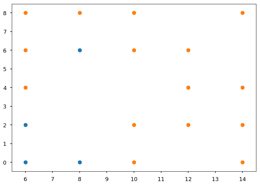
Now we have to repeat the procedure for the branch $[4, 15]$
Lets take a look what points are left

plt.xlim([5.5, 14.5])

plt.scatter(*blue_train.T)
plt.scatter(*orange_train.T);

png

Check $x$ maximum information gain ratio

Nb = 4
No = 15

splits = {"6": (2, 3), "8": (4, 4), "10": (4, 8), "12": (4, 11)}

for threshold, (no, nb) in splits.items():
  print("Threshold = {}\t -> {}".format(threshold, info_gain(Nb, No, no, nb)))

Threshold = 6    -> 0.051004839414443226
Threshold = 8    -> 0.32143493796317624
Threshold = 10   -> 0.16251125329718286
Threshold = 12   -> 0.08198172064120202

print("Information gain ratio with x > 8:",
      info_gain(Nb, No, *splits["8"]) / entropy(5, 3, 4, 3, 4))

Information gain ratio with x > 8: 0.14010311259651076

Check $y$ maximum information gain ratio

Nb = 4
No = 15

splits = {"0": (2, 2), "2": (3, 5), "4": (3, 6), "6": (4, 9)}

for threshold, (no, nb) in splits.items():
  print("Threshold = {}\t -> {}".format(threshold, info_gain(Nb, No, no, nb)))

Threshold = 0    -> 0.08471690647404045
Threshold = 2    -> 0.08617499693494635
Threshold = 4    -> 0.06066554625879636
Threshold = 6    -> 0.13320381570773476

print("Information gain ratio with y > 6:",
      info_gain(Nb, No, *splits["6"]) / entropy(4, 4, 3, 4, 4))

Information gain ratio with y > 6: 0.05757775370755489

Once again $x$ is a winner
And we have a new node

tree = Digraph()

tree.edge("x > 4?\n[15, 15]", "blue\n[11, 0]", "No")
tree.edge("x > 4?\n[15, 15]", "x > 8?\n[4, 15]", "Yes")

tree.edge("x > 8?\n[4, 15]", "[4, 4]", "No")
tree.edge("x > 8?\n[4, 15]", "orange\n[0, 11]", "Yes")

tree

svg

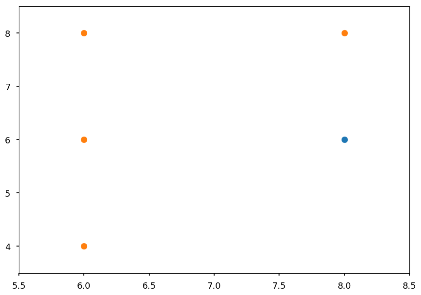
Branch x<= 8¶

We will continue until the tree is fully grown

plt.xlim([5.5, 8.5])

plt.scatter(*blue_train.T)
plt.scatter(*orange_train.T);

png

Again, the best cut may be pretty obvious, but lets check the math
We have one possible cut in $x$

Nb = 4
No = 4

print("Information gain ratio with x > 6:",
      info_gain(Nb, No, 2, 3) / entropy(5, 3))

Information gain ratio with x > 6: 0.05112447853477686

And usual threshold candidates in $y$

splits = {"0": (2, 0), "2": (3, 0), "4": (3, 1), "6": (4, 2)}

for threshold, (no, nb) in splits.items():
  print("Threshold = {}\t -> {}".format(threshold, info_gain(Nb, No, no, nb)))

Threshold = 0    -> 0.31127812445913283
Threshold = 2    -> 0.5487949406953986
Threshold = 4    -> 0.1887218755408671
Threshold = 6    -> 0.31127812445913283

print("Information gain ratio with y > 2:",
      info_gain(Nb, No, *splits["2"]) / entropy(2, 1, 1, 2, 2))

Information gain ratio with y > 2: 0.24390886253128827

And the tree is growing

tree = Digraph()

tree.edge("x > 4?\n[15, 15]", "blue\n[11, 0]", "No")
tree.edge("x > 4?\n[15, 15]", "x > 8?\n[4, 15]", "Yes")

tree.edge("x > 8?\n[4, 15]", "y > 2?\n[4, 4]", "No")
tree.edge("x > 8?\n[4, 15]", "orange\n[0, 11]", "Yes")

tree.edge("y > 2?\n[4, 4]", "blue\n[3, 0]", "No")
tree.edge("y > 2?\n[4, 4]", "[1, 4]", "Yes")

tree

svg

Branch y > 2¶

plt.xlim([5.5, 8.5])
plt.ylim([3.5, 8.5])

plt.scatter(*blue_train.T)
plt.scatter(*orange_train.T);

png

Nb = 1
No = 4

print("Information gain ratio with x > 6:",
      info_gain(Nb, No, 0, 3) / entropy(3, 2))

Information gain ratio with x > 6: 0.33155970728682876

print("Information gain ratio with y > 4:",
      info_gain(Nb, No, 0, 1) / entropy(1, 2, 2))

print("Information gain ratio with y > 6:",
      info_gain(Nb, No, 1, 2) / entropy(1, 2, 2))

Information gain ratio with y > 4: 0.047903442721748145
Information gain ratio with y > 6: 0.11232501392736344

The final tree¶

tree = Digraph()

tree.edge("x > 4?\n[15, 15]", "blue\n[11, 0]", "No")
tree.edge("x > 4?\n[15, 15]", "x > 8?\n[4, 15]", "Yes")

tree.edge("x > 8?\n[4, 15]", "y > 2?\n[4, 4]", "No")
tree.edge("x > 8?\n[4, 15]", "orange\n[0, 11]", "Yes")

tree.edge("y > 2?\n[4, 4]", "blue\n[3, 0]", "No")
tree.edge("y > 2?\n[4, 4]", "x > 6?\n[1, 4]", "Yes")

tree.edge("x > 6?\n[1, 4]", "orange\n[0, 3]", "No")
tree.edge("x > 6?\n[1, 4]", "y > 6?\n[1, 1]", "Yes")

tree.edge("y > 6?\n[1, 1]", "blue\n[1, 0]", "No")
tree.edge("y > 6?\n[1, 1]", "orange\n[0, 1]", "Yes")

tree

svg

It is likely that this tree is overfitted
We will proceed with pruning as it was explained
But first lets implement decision rules to measure accuracy

def tree_nominal(x, y):
  """Implementation of above tree"""
  if x <= 4:
    return "blue"
  elif x > 8:
    return "orange"
  elif y <= 2:
    return "blue"
  elif x <= 6:
    return "orange"
  else:
    return "orange" if y > 6 else "blue"

Sanity check¶

If the tree is built correctly we expect 100% accuracy on training set

for x, y in blue_train:
  print(tree_nominal(x, y), end=' ')

blue blue blue blue blue blue blue blue blue blue blue blue blue blue blue

for x, y in orange_train:
  print(tree_nominal(x, y), end=' ')

orange orange orange orange orange orange orange orange orange orange orange orange orange orange orange

Accuracy before pruning¶

def accuracy(samples, tree):
  """Just print the result of classification"""
  for x, y in samples:
    print("({}, {}) -> {}".format(x, y, tree(x, y)))

accuracy(blue_valid, tree_nominal)

(0, 6) -> blue
(2, 4) -> blue
(4, 0) -> blue
(4, 8) -> blue
(8, 2) -> blue

accuracy(orange_valid, tree)

(8, 4) -> blue
(10, 4) -> orange
(12, 0) -> orange
(12, 8) -> orange
(14, 6) -> orange

Pruning I¶

We want to prune last decision node $y > 6$
In general, majority decides about the leaf node class
As it is a tie here, lets check both

def tree_prune01a(x, y):
  """Implementation of above tree"""
  if x <= 4:
    return "blue"
  elif x > 8:
    return "orange"
  elif y <= 2:
    return "blue"
  elif x <= 6:
    return "orange"
  else:
    return "blue"

def tree_prune01b(x, y):
  """Implementation of above tree"""
  if x <= 4:
    return "blue"
  elif x > 8:
    return "orange"
  elif y <= 2:
    return "blue"
  else:
    return "orange"

accuracy(blue_valid, tree_prune01a)

(0, 6) -> blue
(2, 4) -> blue
(4, 0) -> blue
(4, 8) -> blue
(8, 2) -> blue

accuracy(orange_valid, tree_prune01a)

(8, 4) -> blue
(10, 4) -> orange
(12, 0) -> orange
(12, 8) -> orange
(14, 6) -> orange

Pruning does not change the accuracy
We always use Occam's razor and prune01a is preferred over nominal tree
But lets see how prune01b works

accuracy(blue_valid, tree_prune01b)

(0, 6) -> blue
(2, 4) -> blue
(4, 0) -> blue
(4, 8) -> blue
(8, 2) -> blue

accuracy(orange_valid, tree_prune01b)

(8, 4) -> orange
(10, 4) -> orange
(12, 0) -> orange
(12, 8) -> orange
(14, 6) -> orange

In this case we even get the increase of the accuracy
We decide to prune a tree by replacing $y > 6$ decision node with "orange" leaf node
Which automatically removes $x > 6$ decision node

tree = Digraph()

tree.edge("x > 4?\n[15, 15]", "blue\n[11, 0]", "No")
tree.edge("x > 4?\n[15, 15]", "x > 8?\n[4, 15]", "Yes")

tree.edge("x > 8?\n[4, 15]", "y > 2?\n[4, 4]", "No")
tree.edge("x > 8?\n[4, 15]", "orange\n[0, 11]", "Yes")

tree.edge("y > 2?\n[4, 4]", "blue\n[3, 0]", "No")
tree.edge("y > 2?\n[4, 4]", "orange\n[1, 4]", "Yes")

tree

svg

Pruning II¶

Now, lets see the accuracy after removing $y > 2$ node
It is once again a tie, so lets check both scenarios

def tree_prune02a(x, y):
  """Implementation of above tree"""
  if x <= 4:
    return "blue"
  else:
    return "orange"

def tree_prune02b(x, y):
  """Implementation of above tree"""
  if x <= 4:
    return "blue"
  elif x > 8:
    return "orange"
  else:
    return "blue"

accuracy(blue_valid, tree_prune02a)

(0, 6) -> blue
(2, 4) -> blue
(4, 0) -> blue
(4, 8) -> blue
(8, 2) -> orange

accuracy(orange_valid, tree_prune02a)

(8, 4) -> orange
(10, 4) -> orange
(12, 0) -> orange
(12, 8) -> orange
(14, 6) -> orange

accuracy(blue_valid, tree_prune02b)

(0, 6) -> blue
(2, 4) -> blue
(4, 0) -> blue
(4, 8) -> blue
(8, 2) -> blue

accuracy(orange_valid, tree_prune02b)

(8, 4) -> blue
(10, 4) -> orange
(12, 0) -> orange
(12, 8) -> orange
(14, 6) -> orange

In both cases the error increased
We stop pruning and leave the tree as it is in prune01b version

Summary¶

C4.5 algorithm gives the full and clear prescription for building decision trees
It may look as a long procedure, but it is only because I wanted to show everything step by step and avoid "after a few trivial steps..."
ID3/C4.5/C5.0 are based on information theory
There is alternative procedure based on gini impurity, which is used by CART

CART¶

CART stands for Classification and Regression Tree
It was created independently from ID3 (more or less at the same time)
The main differences:
- it creates binary trees (each decision node has two branches)
- it uses gini impurity instead of information gain
- it supports numerical target variables (regression)

Gini impurity¶

Let $T = \{T_1, T_2, ..., T_n\}$ be the set of $n$ classes
and $P = \{p_1, p_2, ..., p_n\}$ be the probability distribution
where $p_i$ is the probability that a sample belongs to class $T_i$
and $1 - p_i$ is the probability that it belongs to another class
Gini impurity is defines as
$I(P) = \sum\limits_{i=1}^n p_i\cdot (1 - p_i) = \sum\limits_{i=1}^n p_i - \sum\limits_{i=1}^n p_i^2 = 1 - \sum\limits_{i=1}^n p_i^2$
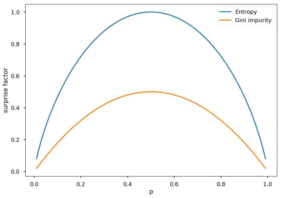
As before (for entropy), lets consider two case scenario with $P = (p, 1 - p)$ , so gini impurity is given by $I = 1 - p^2 - (1 - p)^2 = -2p(p - 1)$

p = np.arange(0.01, 1.0, 0.01)

plt.xlabel("p")
plt.ylabel("surprise factor")

plt.plot(p, -p * np.log2(p) - (1 - p) * np.log2(1 - p), label="Entropy");
plt.plot(p, -2*p*(p - 1), label="Gini impurity")

plt.legend();

png

Play Golf¶

Lets consider once again Play Golf dataset

import pandas as pd

# first row = headers
src = "http://chem-eng.utoronto.ca/~datamining/dmc/datasets/weather_nominal.csv"

golf_data = pd.read_csv(src)

golf_data

	Outlook	Temperature	Humidity	Windy	Play golf
0	Rainy	Hot	High	False	No
1	Rainy	Hot	High	True	No
2	Overcast	Hot	High	False	Yes
3	Sunny	Mild	High	False	Yes
4	Sunny	Cool	Normal	False	Yes
5	Sunny	Cool	Normal	True	No
6	Overcast	Cool	Normal	True	Yes
7	Rainy	Mild	High	False	No
8	Rainy	Cool	Normal	False	Yes
9	Sunny	Mild	Normal	False	Yes
10	Rainy	Mild	Normal	True	Yes
11	Overcast	Mild	High	True	Yes
12	Overcast	Hot	Normal	False	Yes
13	Sunny	Mild	High	True	No

Gini impurity¶

We treat all values as they are continues
And consider all possible split
Every split leads to two subsets $S_1$ and $S_2$
And gini impurity for a set $S$ for given split is given by:
$I(S) = \frac{|S_1|}{|S|}\cdot I(S_1) + \frac{|S_2|}{|S|}\cdot I(S_2)$

def gini(*distribution):
  """Calculate gini impurity for given ditribution of samples"""
  sum2 = sum(distribution)**2  # normalization factor

  return 1 - sum([p**2 for p in distribution])/sum2

def gini_split(s1, s2, g1, g2):
  """Calcualte impurity for given split

  s1 -- the size of S1 subset
  s1 -- the size of S2 subset
  g1 -- I(S1)
  g2 -- I(S2)
  """
  s = s1 + s2  # the total set size

  return s1/s * g1 + s2/s * g2

            | Play golf |
            =============
            | yes | no  |
      -------------------
      | yes |  2  |  3  | 5
rainy | no  |  7  |  2  | 9
      -------------------
               9     5

gini_split(5, 9, gini(2, 3), gini(7, 2))

0.3936507936507937

            | Play golf |
            =============
            | yes | no  |
      -------------------
      | yes |  3  |  2  | 5
sunny | no  |  6  |  3  | 9
      -------------------
               9     5

gini_split(5, 9, gini(3, 2), gini(6, 3))

0.45714285714285713

               | Play golf |
               =============
               | yes | no  |
         -------------------
         | yes |  4  |  0  | 4
overcast | no  |  5  |  5  | 10
         -------------------
                  9     5

gini_split(4, 10, gini(4, 0), gini(5, 5))

0.35714285714285715

From Outlook feature the best choice is Overcast as it minimizes impurity
However, we would have to check other features and choose the best predictor from all possibilities
We have one step by step example done though
So lets use some tool

Scikit learn¶

One step by step example is behind us, so now lets use some tool
CART is implemented in scikit-learn
However, their implementation takes only numerical values
So we will use LabelDecoder to convert all values to numbers

from sklearn.preprocessing import LabelEncoder

# pandas.DataFrame.apply applies a function to given axis (0 by default)
# LabelEncoder encodes class labels with values between 0 and n-1
golf_data_num = golf_data.apply(LabelEncoder().fit_transform)

golf_data_num

	Outlook	Temperature	Humidity	Windy	Play golf
0	1	1	0	0	0
1	1	1	0	1	0
2	0	1	0	0	1
3	2	2	0	0	1
4	2	0	1	0	1
5	2	0	1	1	0
6	0	0	1	1	1
7	1	2	0	0	0
8	1	0	1	0	1
9	2	2	1	0	1
10	1	2	1	1	1
11	0	2	0	1	1
12	0	1	1	0	1
13	2	2	0	1	0

Now, lets splits our dataset to features and labels

# DataFrame.iloc makes an access thourgh indices
# we want all rows and first 4 columns for features
# and the last column for labels
data = np.array(golf_data_num.iloc[:, :4])
target = np.array(golf_data_num.iloc[:, 4])

Once data is prepared, creating a tree is as easy as 2 + 2 -1

from sklearn import tree

golf_tree = tree.DecisionTreeClassifier()

golf_tree.fit(data, target);

sklearn.tree supports drawing a tree using graphviz

import graphviz

# dot is a graph description language
dot = tree.export_graphviz(golf_tree, out_file=None, 
                           feature_names=golf_data.columns.values[:4],  
                           class_names=["no", "yes"],  
                           filled=True, rounded=True,  
                           special_characters=True) 

# we create a graph from dot source using graphviz.Source
graph = graphviz.Source(dot) 
graph

svg

Please note, that in the case of a real problem we would want to have a validation set and perform a pruning (scikit-learn does not support it though)

Regression¶

The difference now is that targets are numerical values (instead of categorical), e.g. in golf data - number of hours played instead of "yes / no"
Features may be either discrete or continuous
The idea is the same though - we want to create a binary tree and minimize the error on in each leaf
However, having continuous values as targets we can not simply use entropy or gini
We need to use different measurement - variance
$V(X) = \frac{1}{n}\sum\limits_{i=1}^n (x_i - \bar x)^2$
where $X = \{x_1, ..., x_n\}$ and $\bar x$ is the average value
Note, that here $x_i$ are equally likely

Simple example¶

Before we learn how to grow a regression tree, lets take a look how it works on a simple example
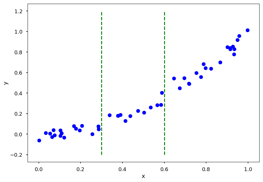
Lets consider data distributed according to $x^2$ (with some noise, obviously)
It means with have continuous features ( $x$ ) and targets ( $y$ )
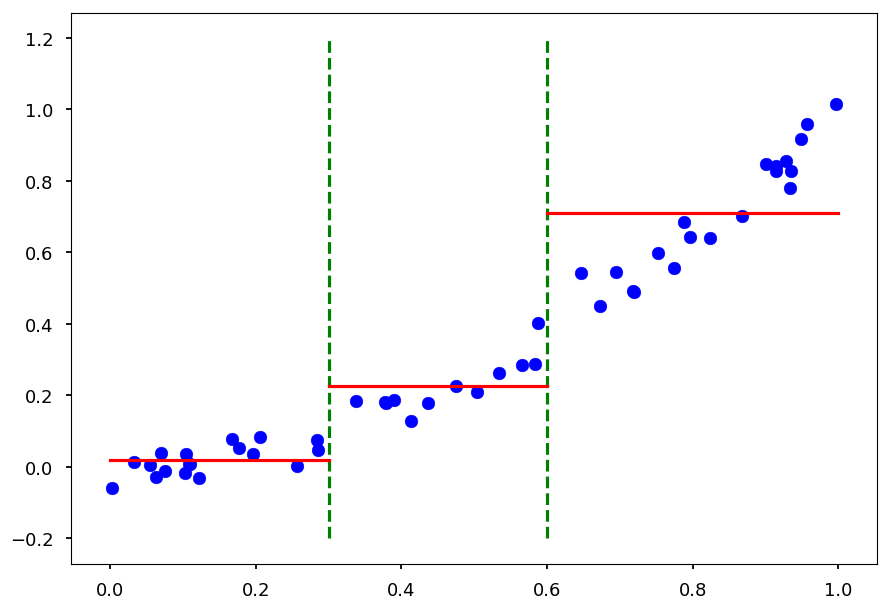
We will split by hand the domain in $0.3$ and $0.6$

X = np.random.sample(50)
Y = np.array([x**2 + np.random.normal(0, 0.05) for x in X])

plt.xlabel("x")
plt.ylabel("y")

plt.scatter(X, Y, color='b')
plt.plot([0.3, 0.3], [-0.2, 1.2], 'g--')
plt.plot([0.6, 0.6], [-0.2, 1.2], 'g--');

png

The corresponding tree would look like this

tree = Digraph()

tree.edge("x < 0.3?", "?", "No")
tree.edge("x < 0.3?", "x < 0.6?", "Yes")

tree.edge("x < 0.6?", "? ", "No")
tree.edge("x < 0.6?", "?  ", "Yes")

tree

svg

For each split lets find a value $\bar y$

def avg(X, Y, x_min, x_max):
  """Return the average value in (x_min, x_max) range"""
  n = 0    # number of samples in given split 
  avg = 0  # average value

  for x, y in zip(X, Y):
    if x >= x_min and x < x_max:
      n += 1
      avg += y

  return avg / n

plt.scatter(X, Y, color='b')

plt.plot([0.3, 0.3], [-0.2, 1.2], 'g--')
plt.plot([0.6, 0.6], [-0.2, 1.2], 'g--')

y = avg(X, Y, 0, 0.3)
plt.plot([0.0, 0.3], [y, y], 'r')

y = avg(X, Y, 0.3, 0.6)
plt.plot([0.3, 0.6], [y, y], 'r')

y = avg(X, Y, 0.6, 1)
plt.plot([0.6, 1.0], [y, y], 'r');

png

Alternatively, one could do linear regression for split

Growing a tree¶

The idea is similar as for numerical values in classification problems
For each feature we check all possible splits and calculate variance
We choose a binary split which minimzes variance

from sklearn.tree import DecisionTreeRegressor

# create a decision tree regressor
fit = DecisionTreeRegressor()

# and grow it (note that X must be reshaped)
fit.fit(np.reshape(X, (-1, 1)), Y);

# prepare test sample with "newaxis" trick
X_test = np.arange(0.0, 1.0, 0.01)[:, np.newaxis]
Y_test = fit.predict(X_test)

plt.scatter(X, Y, color='b')
plt.plot(X_test, Y_test);

png

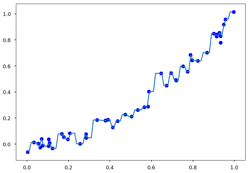
And this is a perfect example of overfitting
Each point was classified as a separate target
Beacause without any stopping criterion the tree is growing until there is a single point in a leaf
There are several strategies to pre-prune a tree:
- define a max depth of a tree
- define a minimum number of samples in a leaf
- define a minimum impurity
- define a minimum impurity decrease
Whatever method is chosen you get a hyperparameter
And we already know how to find an optimal hyperparameter: cross-validation

Tree: cross-validation¶

To make it easier to check all possible methods lets create a simple class to do that for us
It takes training data and hyperparameter name (as named in scikit-learn)
It can change hyperparameter
It can perform a cross-validation for a set of hyperparameter values
It can make accuracy and best fit plots

from sklearn.model_selection import cross_val_score
from sklearn.tree import DecisionTreeRegressor

class TreeCV:
  """Perform a cross-validation for chosen hyperparameter"""

  def __init__(self, X, Y, hp="max_depth"):
    """Save training data"""
    self.X = X    # features
    self.Y = Y    # targets
    self.hp = hp  # hyperparameter


  def set_method(self, hp):
    """Set hyperparameter to use"""
    self.hp = hp


  def cross_me(self, *hp_vals):
    """Perform cross validation for given hyperparameter values"""
    self.scores = []  # the accuracy table
    self.best = None  # the best fit

    best_score = 0

    for hp in hp_vals:
      # create a tree with given hyperparameter cut
      fit = DecisionTreeRegressor(**{self.hp: hp})

      # calculate a cross validation scores and a mean value
      score = cross_val_score(fit, np.reshape(X, (-1, 1)), Y).mean()

      # update best fit if necessary
      if score > best_score:
        self.best = fit
        best_score = score

      self.scores.append([hp, score])

    # train the best fit
    self.best.fit(np.reshape(X, (-1, 1)), Y)


  def plot(self):
    """Plot accuracy as a function of hyperparameter values and best fit"""
    plt.figure(figsize=(15, 5))

    plt.subplot(1, 2, 1)

    plt.xlabel(self.hp)
    plt.ylabel("accuracy")

    plt.plot(*zip(*self.scores))

    plt.subplot(1, 2, 2)

    X_test = np.arange(0.0, 1.0, 0.01)[:, np.newaxis]
    Y_test = self.best.predict(X_test)

    plt.scatter(self.X, self.Y, color='b', marker='.', label="Training data")
    plt.plot(X_test, X_test * X_test, 'g', label="True distribution")    
    plt.plot(X_test, Y_test, 'r', label="Decision tree")

    plt.legend()

Traning dataset¶

X = np.random.sample(200)
Y = np.array([x**2 + np.random.normal(0, 0.05) for x in X])

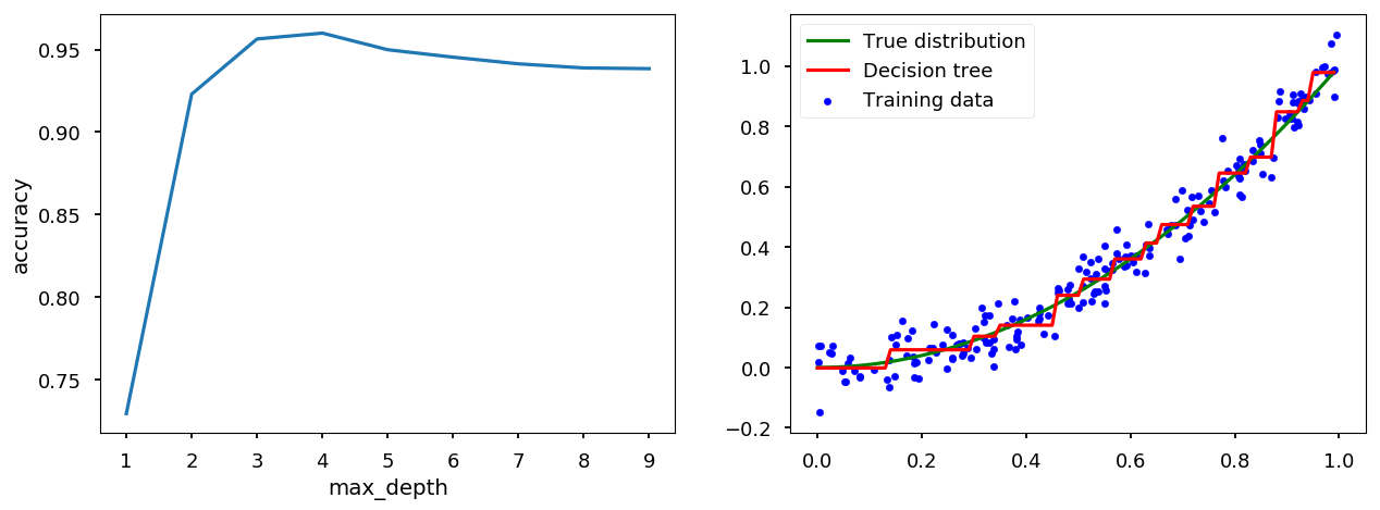
`max_depth`¶

tree_handler = TreeCV(X, Y)
tree_handler.cross_me(*range(1, 10))
tree_handler.plot()

png

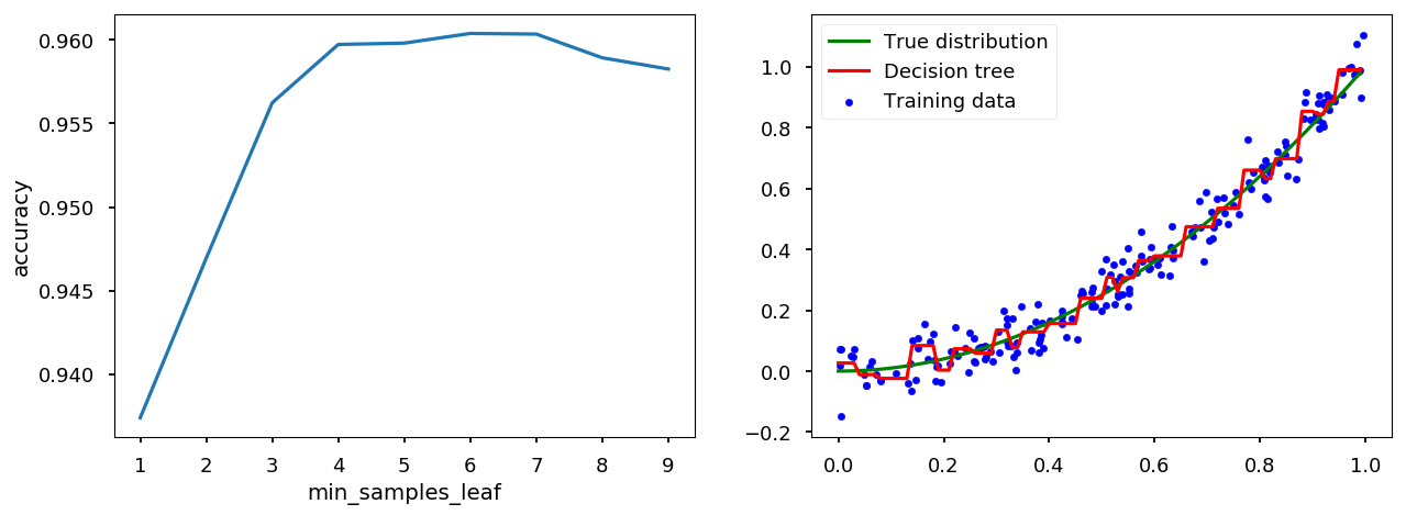
`min_samples_leaf`¶

tree_handler.set_method("min_samples_leaf")
tree_handler.cross_me(*range(1, 10))
tree_handler.plot()

png

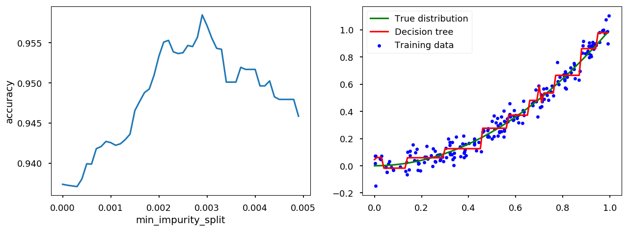
`min_impurity_split`¶

# min_impurity_split is depracated so lets disable warnings
import warnings
warnings.filterwarnings("ignore", category=DeprecationWarning)

tree_handler.set_method("min_impurity_split")
tree_handler.cross_me(*np.arange(0.0, 5e-3, 1e-4))
tree_handler.plot()

png

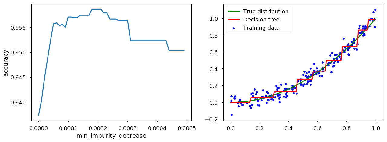
`min_impurity_decrease`¶

tree_handler.set_method("min_impurity_decrease")
tree_handler.cross_me(*np.arange(0.0, 5e-4, 1e-5))
tree_handler.plot()

png

Bias-Variance trade-off¶

        +================+================+
       /\                |                /\
      /  \               |               /  \
     /    \              |              /    \
    /      \             |             /      \
   /        \            |            /        \
  / variance \           |           /   bias   \
  ^^^^^^^^^^^^           |           ^^^^^^^^^^^^
                         |
                         |
                         |
overfitting   <----------+--------->   underfitting

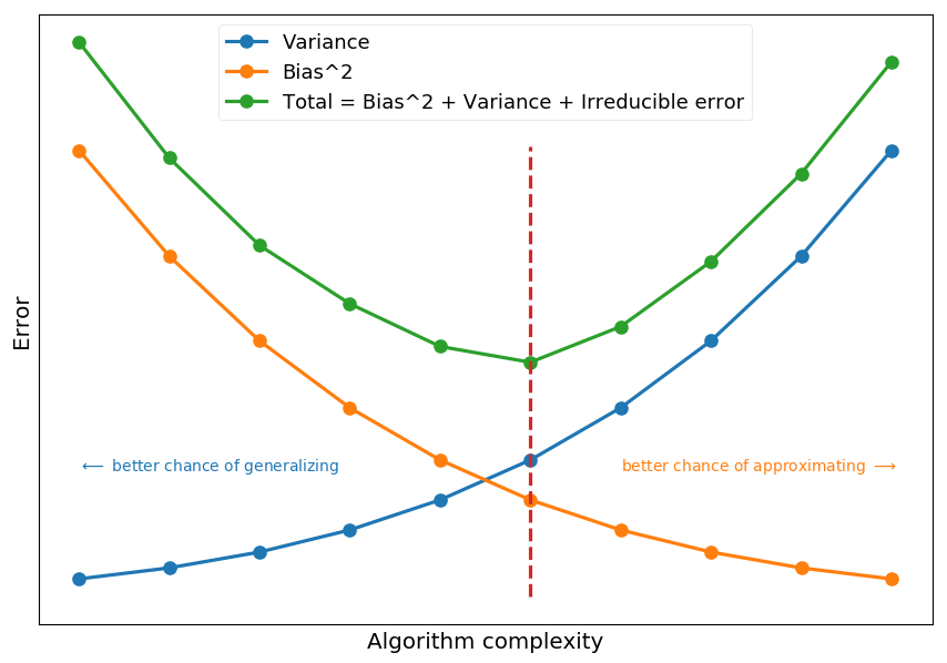
Bias is an error coming from wrong model assumptions, which do not allow an algorithm to learn all patterns from training data.
Variance is an error coming from sensivity to features specific for training data.
High bias leads to underfitting and high variance to overfitting.
Total error also depends on irreducible error (noise that can not be reduced by algorithm)
Ultmiate goal is to minimize the total error

# fake bias, variance and noise
complexity = np.arange(1, 2, 0.1)
variance = np.power(complexity, 5)
bias2 = variance[::-1]
irreducible = [10*np.random.normal(abs(x - 1.5), 0.01) for x in complexity]

# total error = variance + bias^2 + irreducible
total = variance + bias2 + irreducible

plt.xticks([])
plt.yticks([])

plt.xlabel("Algorithm complexity")
plt.ylabel("Error")

plt.plot(complexity, variance, 'C0o-', label='Variance')
plt.plot(complexity, bias2, 'C1o-', label="Bias^2")
plt.plot(complexity, total, 'C2o-', label="Total = Bias^2 + Variance + Irreducible error")

plt.plot([1.5, 1.5], [0, 25], 'C3--')

plt.text(1.0, 7, "$\longleftarrow$ better chance of generalizing", color='C0')
plt.text(1.6, 7, "better chance of approximating $\longrightarrow$", color='C1')

plt.legend();

png

Decision trees are sensitive to splits - small changes in training data may change a tree structure
- deep trees tend to have high variance and low bias
- shallow trees tend to have low variance and high bias

Quick math¶

Basic¶

The general goal of regression is to find how some dependent variable (target, $y$ ) is changing when independent variable (feature, $x$ ) varies
Lets assume there is some true relationship describing this dependence $y = f(x)$
We want to find $f(x)$ from observations of $(x, y)$ pairs
Although, in real life we get some noisy observation, so $y = f(x) + \epsilon$
As we do not know function $f(x)$ we want to approximate it with some other function $g(x)$ (estimator)
In general, $g(x)$ is a parametrized model which can take many possible functional form
- e.g. $g(x) = a\cdot x^2 + b\cdot x + c$ can take different coefficients (based on a training dataset)

Bias and variance¶

Lets imagine there are $N$ possible training datasets $\{D_1, D_2, ..., D_N\}$
For a given dataset one gets an estimators $g^{(D)}(x)$
Lets denote the expected estimator by $\mathbf{E}_{D}\left[g^{(D)}(x)\right] \equiv \bar g(x)$
If $N$ is large we can approximate it by an average over all datasets (law of large numbers)

$\bar g(x) \approx \frac{1}{N}\sum\limits_{i=1}^N g^{(D_i)}(x)$
The variance of an estimator tells us how far particular predictions are from the mean value

$var = \mathbf{E}_{D}\left[\left(g^{(D)}(x) - \bar g(x)\right)^2\right]$
Thus, if the training does not depend on the choice of a dataset the variance is low
The bias of an estimator tells us how far the mean value is from the true value

$bias = \bar g(x) - f(x)$
Thus, if the model decribes data accurately the bias is low
Please note the hidden assumption that all possible values of $x$ are equally likely

Goodness of a model¶

The common practice to determine the goodness of a model fit is to calculate mean squared error
The mean squared error is, well, the mean value of error squared:

$mse = \mathbf{E}_{x}\left[\mathbf{E}_{D}\left[\left(g^{(D)}(x) - y\right)^2\right]\right]$
Lets consider MSE for a particlar point $x$ , $y = f(x) + \epsilon$ , so

$mse = \mathbf{E}_{D}\left[\left(g^{(D)}(x) - y\right)^2\right] = \mathbf{E}_{D}\left[\left(g^{(D)}(x)\right)^2\right]- 2\cdot\mathbf{E}_{D}\left[g^{(D)}(x)\cdot y\right] + \mathbf{E}_{D}\left[y^2\right]$
Here, we used the linearity of the expected value operator. Lets use another common property: $\mathbf{E}\left[X^2\right] = \mathbf{E}\left[\left(X - \mathbf{E}\left[X\right]\right)^2\right] + \mathbf{E}\left[X\right]^2$
So the first term can be rewritten in the form

$\mathbf{E}_{D}\left[\left(g^{(D)}(x)\right)^2\right] = \mathbf{E}_{D}\left[\left(g^{(D)}(x) - \mathbf{E}_{D}\left[g^{(D)}(x)\right]\right)^2\right] + \mathbf{E}_{D}\left[g^{(D)}(x)\right]^2 = \mathbf{E}_{D}\left[\left(g^{(D)}(x) - \bar g(x)\right)^2\right] + \left(\bar g(x)\right)^2$
And the last term

$\mathbf{E}_{D}\left[y^2\right] = \mathbf{E}_{D}\left[\left(y - \mathbf{E}_{D}\left[y\right]\right)^2\right] + \mathbf{E}_{D}\left[y\right]^2 = \mathbf{E}_{D}\left[\left(y - f(x)\right)^2\right] + \left(f(x)\right)^2$
Here, we used the fact that $\mathbf{E}_{D}\left[y\right] = f(x)$ (noise would average out when averaging over infinite number of datasets)
For the middle term we use the fact that for independent $X$ and $Y$ : $\mathbf{E}\left[XY\right] = \mathbf{E}\left[X\right]\cdot\mathbf{E}\left[Y\right]$ , so $\mathbf{E}_{D}\left[g^{(D)}(x)\cdot y\right] = \bar g(x)\cdot f(x)$
Taking all together we get

$mse = \underbrace{\mathbf{E}_{D}\left[\left(g^{(D)}(x) - \bar g(x)\right)^2\right]}_{variance} + \underbrace{\left(\bar g(x) - f(x)\right)^2}_{bias^2} + \underbrace{\mathbf{E}_{D}\left[\left(y - f(x)\right)^2\right]}_{noise}$

Example¶

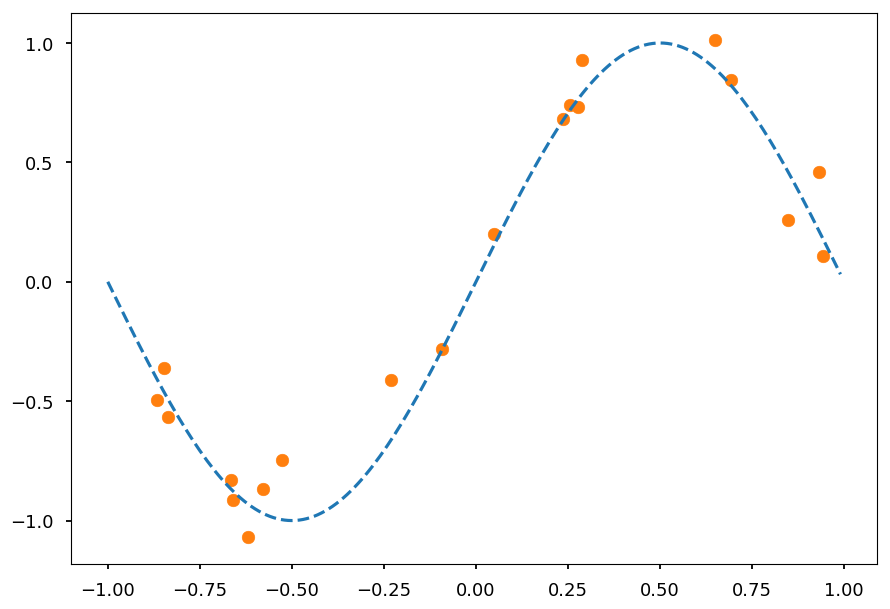
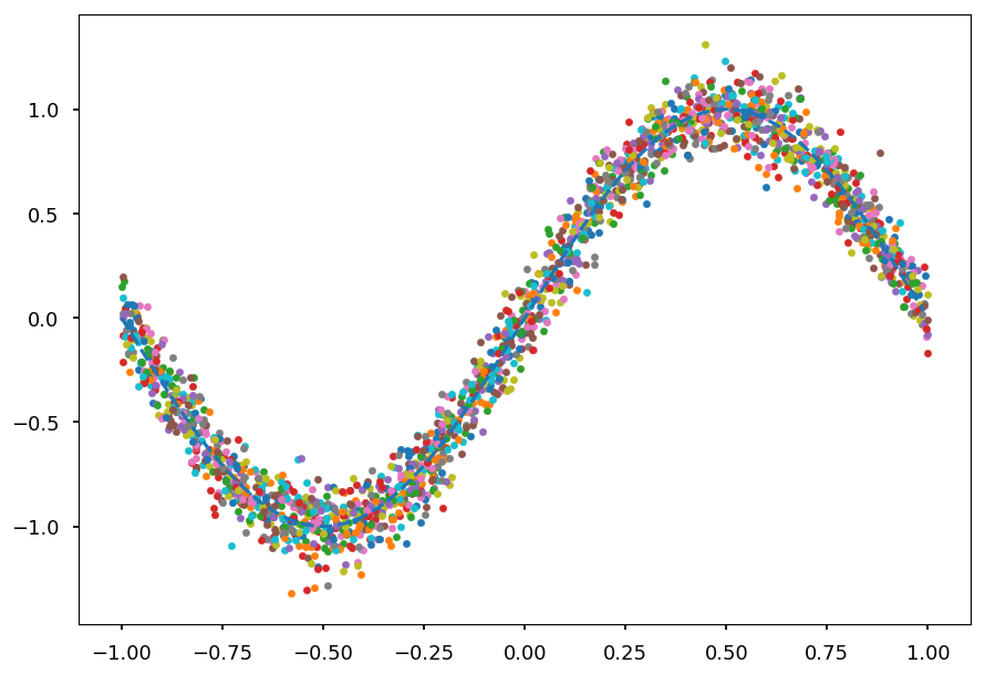
Lets consider $f(x) = \sin(\pi x)$
With a noise given by a zero-mean Gaussian with a variance $\sigma^2$
So the observation $y = f(x) + \mathcal{N}(0, \sigma^2)$

from math import sin, cos, pi, exp

def get_dataset(N=20, sigma=0.1):
  """Generate N training samples"""
  # X is a set of random points from [-1, 1]
  X = 2 * np.random.sample(N) - 1
  # Y are corresponding target values (with noise included)
  Y = np.array([sin(pi*x) + np.random.normal(0, sigma) for x in X])

  return X, Y

# plot a sample
X, Y = get_dataset()

x_ = np.arange(-1, 1, 0.01)

plt.scatter(X, Y, color='C1')
plt.plot(x_, np.sin(np.pi * x_), 'C0--');

png

We do not know $f(x)$
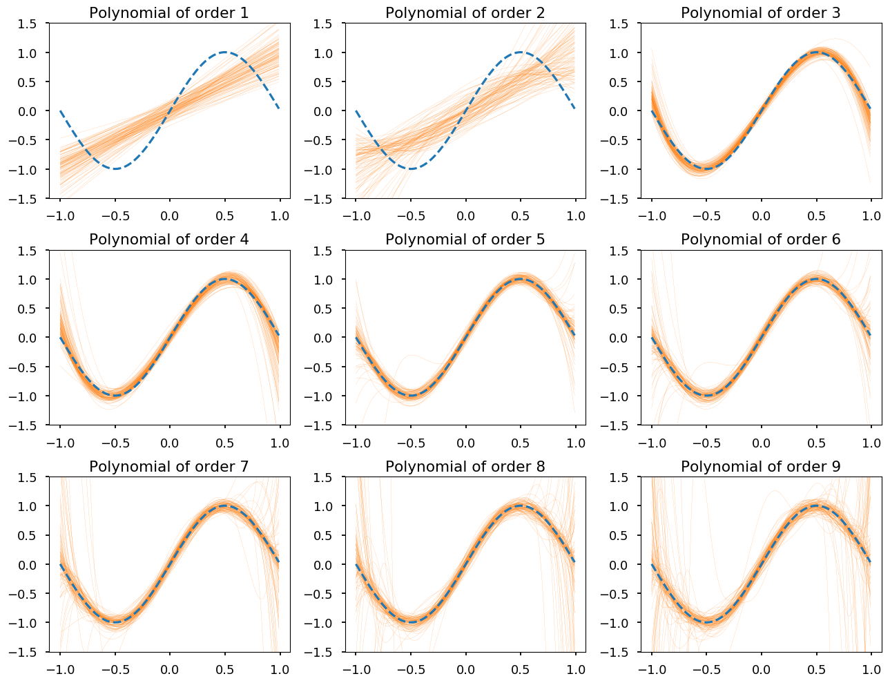
We assume it is a polynomial
Lets consider polynomials of orders: $1 - 9$
- $g_1(x) = a_1\cdot x + a_0$
- $g_2(x) = a_2\cdot x^2 + \cdots + a_0$
- $g_3(x) = a_3\cdot x^3 + \cdots + a_0$
- ...
Lets assume we have 100 independent dataset
Each one has 20 points $(x, y = \sin(\pi x) + \mathcal{N}(0, \sigma^2))$

# generate 100 datasets with default settings
datasets = [get_dataset() for i in range(100)]

# and plot them all together with true signal
for i in range(100):
  plt.scatter(datasets[i][0], datasets[i][1], marker='.')

plt.plot(x_, np.sin(np.pi * x_), 'C0--');

png

Now we need to fit each polynomial to each dataset separately

def get_fit(N, data):
  """Find a fit of polynomial of order N to data = (X, Y)"""
  return np.poly1d(np.polyfit(data[0], data[1], N))

# for the whole range of possible polynomials orders
# create a list of fits to different datasets
fits = [[get_fit(order, data) for data in datasets] for order in range(1, 10)]

plt.figure(figsize=(13, 10))

for order in range(1, 10):
  plt.subplot(3, 3, order)
  plt.ylim([-1.5,1.5])

  for g in fits[order - 1]:
    plt.plot(x_, g(x_), 'C1-', linewidth=0.1)

  plt.plot(x_, np.sin(np.pi * x_), 'C0--')

  plt.title("Polynomial of order {}".format(order));

plt.tight_layout();

png

Training and test errors¶

In real life is impossible (unless one creates data by hand) to calculate true variance and bias
One would need all possible datasets $D$ and all possible input values $x$
Thus, usually one looks at training and test errors
- Training error is measured on the data used to make a fit
- Test/validation error is measured on unseen data

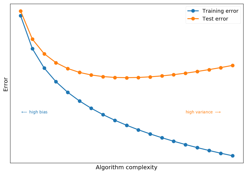
# fake error
complexity = np.arange(0.1, 2, 0.1)
train_error = -np.log(complexity)
test_error = -np.log(complexity) + np.power(complexity, 1)

plt.xticks([])
plt.yticks([])

plt.xlabel("Algorithm complexity")
plt.ylabel("Error")

plt.plot(complexity, train_error, 'C0o-', label='Training error')
plt.plot(complexity, test_error, 'C1o-', label="Test error")

plt.text(0.1, 0.25, "$\longleftarrow$ high bias", color='C0')
plt.text(1.5, 0.25, "high variance $\longrightarrow$", color='C1')

plt.legend();

png

High training error indicates high bias (which means underfitting)
Training error must decrease with model complexity
If the training error is high:
- Use more complex model (or new model architecture)
- Use more features - maybe there is just not enough information to make a good prediction
- Train longer (if the algorithm is an iterative optimization problem)
- Decrease regularization (next lecture)
Test error deacreses with model complexity up to a point when algorithm is to sensitive to features seen in training data
If test error starts to increase it indicates high variance (which means overfitting)
If test error is high:
- Use more data - easy to say hard to do...
- Use less features
- Increase regularization
- Use different model

Ensemble learning¶

Lets first define a weak learner as a classifier which is just slighlty better than random guessing
The idea behind ensemble learning is to create a strong learner as a combination of many weak learners
We will discuss two popular ensemble methods:
- Bagging (bootstrap aggregating), e.g. random forest
- Boosting, e.g. boosted decision tress

Random forest¶

Once we know a way to produce a tree we can create a forest
And each tree contributes to a final prediction
It is a random forest, because each tree is randomly incomplete - trained only on a random subsets of samples and features (features bagging)
The final prediction of a random forest is an avearge predictions (for regression) or a majority vote (classification)

Intuitive / naive example¶

Imagine you want to go to a cinema and need to choose a movie to watch
You can ask a friend about the recommendation
- She/he would ask you about movies you watched in the past
- and (based on your answers) create a set of rules (a decision tree)
- to finally recommend you a movie (make a prediction)
Alternatively, you can ask many friends for an advice
- Each friend would ask you random questions to give an answer
- At the end, you choose a movie with most votes

The algorithm¶

Lets imagine we have $N$ samples in our dataset (e.g. $N$ movies you watched)
Each sample has $M$ features (e.g. do you like a movie? do you like the leading actor / actress or director?)
To create a tree take $n$ random samples from the dataset and at each node select $m << M$ features ( $m \sim \sqrt M$ ) to find the best predictor
Repeat the procedure for next trees until you reach desired size of a forest

                    +------------+
                    |            |
                    |   Dataset  |
         +----------+            +----------+
         |          | N features |          |
         |          |            |          |
         v          +------------+          v                    Hyperparameters:

+-----------------+                 +-----------------+
|                 |                 |                 |
| Random subset 1 |      . . .      | Random subset T |
|                 |                 |                 |              - the number of trees
|   N features    |                 |   N features    |              - the size of subsets
|                 |                 |                 |
+--------+--------+                 +--------+--------+
         |                                   |
         v                                   v

+-----------------+                 +-----------------+
|                 |                 |                 |
|     Tree 1      |      . . .      |     Tree T      |
|                 |                 |                 |
+--------+--------+                 +-----------------+
         |
         |          +-------------+          +--------+
         |          |             |          |        |
         +--------> | M1 features +--------> | Node 1 |              - the number of random features
         |          |             |          |        |              - the size of a single tree
         |          +-------------+          +--------+
         |
         |          +-------------+          +--------+
         |          |             |          |        |
         +--------> | M2 features +--------> | Node 2 |
         |          |             |          |        |
         |          +-------------+          +--------+

                           .
                           .
                           .

Boosted trees¶

The idea is similar to bagging
The key differences are:
- Data is reweighted every time a weak learner is added (so future learners focus on misclassified samples)
- The final prediction is weighted average (better classifiers have higher weights)

                            Bagging (parallel)

       +--------------------+                +----------------+
       |                    |                |                |
+----> |      Dataset       +--------------> | Weak learner 1 |
|      |                    |                |                |
|      +--------------------+                +----------------+
|
|
|      +--------------------+                +----------------+
|      |                    |                |                |
+----> |      Dataset       +------------->  | Weak learner 2 |
|      |                    |                |                |
|      +--------------------+       .        +----------------+
|                                   .
|                                   .
|      +--------------------+                +----------------+
|      |                    |                |                |
+----> |      Dataset       +------------->  | Weak learner N |
       |                    |                |                |
       +--------------------+                +----------------+

$\hspace{140pt}\text{output} = \frac{1}{N}\sum \text{output}_i$

                          Boosting (sequential)

      +--------------------+                +----------------+
      |                    |                |                |
      |      Dataset       +--------------> | Weak learner 1 |
      |                    |                |                |
      +--------------------+                +--------+-------+
                                                     |
                +------------------------------------+
                |
                v

      +--------------------+                +----------------+
      |                    |                |                |
      | Reweighted dataset +------------->  | Weak learner 2 |
      |                    |                |                |
      +--------------------+                +--------+-------+
                                                     |
                +------------     . . .      --------+
                |
                v

      +--------------------+                +----------------+
      |                    |                |                |
      | Reweighted dataset +------------->  | Weak learner N |
      |                    |                |                |
      +--------------------+                +----------------+

$\hspace{130pt}\text{output} = \sum w_i\cdot \text{output}_i$

AdaBoost¶

AdaBoost is on of the most famous algorithms in machine learning
Y. Freund and R. Schapire got a Gödel Prize for this
Lets consider $N$ labled training examples $(x_1, y_1), \cdots, (x_N, y_N)$ , where $x_i \in X$ and $y_i = \left\{-1, 1\right\}$
The initial distribution is initizlized with $D_1(i) = \frac{1}{N}$ , where $i = 1, \cdots, N$ (so every sample is equaly likely)
For $t = 1, \cdots, T$ :
- train a weak learner using $D_t$ , $h_t: X \rightarrow \left\{-1, 1\right\}$
- choose the one which minimizes the weighted error
  $\epsilon_t = \sum\limits_{i=1}^{N}D_t(i)\delta\left(h_t(x_i)\neq y_i\right)$
- calculate $\alpha_t$
  $\alpha_t = \frac{1}{2}\ln\left(\frac{1 - \epsilon_t}{\epsilon_t}\right)$
- For $i = 1, \cdots, N$ update weights according to
  $D_{t+1} = \frac{D_t(i)}{Z_t}\begin{cases}e^{-\alpha_t} & h_t(x_i) = y_i \\ e^{\alpha_t} & h_t(x_i) \neq y_i \end{cases} = \frac{D_t(i)}{Z_t}e^{-\alpha_ty_ih_t(x_i)}$
- $Z_t$ is a normilization factor so $D_{t+1}$ is a distribution
  $Z_t = \sum\limits_{i=1}^ND_t(i)e^{-\alpha_ty_ih_t(x_i)}$
The final hyptohesis $H$ is computes the sign of a weighted combination of weak hypotheses
$H(x) = \text{sign}\left(\sum\limits_{t=1}^T\alpha_th_t(x)\right)$

Out-of-bag error¶

Out-of-bag (OOB) error may be used for machine learning models using bootstrap aggregation (like random forest and boosted trees) instead of cross-validation
Bagging involves random sampling with replacement
Some samples are not used in the training process (out-of-bag samples) and therefore can be used to calculate test error
OOB error is the average error over all training samples calculated using predictions from weak classifiers which do not contain particular sample in their bootstrap samples

Example¶

Lets consider some fake data generated with make_blobs from scikit-learn
and then apply decision trees with different maximum depths
and random forests with different maximum depths

Dataset¶

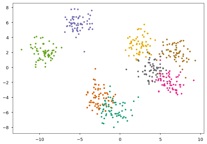
sklearn.datasets.make_blobs allows to generate random Gaussian blobs
We generate 8 blobs with fixed random generator (just to make sure we get the same set every time)

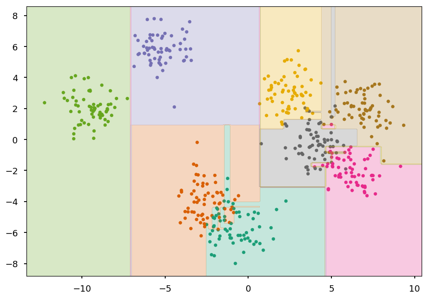
from sklearn.datasets import make_blobs

# generate 5 blobs with fixed random generator
X, Y = make_blobs(n_samples=500, centers=8, random_state=300)

plt.scatter(*X.T, c=Y, marker='.', cmap='Dark2');

png

Train and visualize¶

To make our life easier we create a function to
- plot training data on existing axes or new one (if not provided)
- train given classifier on given dataset
- create countours representing predictions of the classifier

def train_and_look(classifier, X, Y, ax=None, title='', cmap='Dark2'):
  """Train classifier on (X,Y). Plot data and prediction."""
  # create new axis if not provided
  ax = ax or plt.gca();

  ax.set_title(title)

  # plot training data
  ax.scatter(*X.T, c=Y, marker='.', cmap=cmap)

  # train a cliassifier
  classifier.fit(X, Y)

  # create a grid of testing points
  x_, y_ = np.meshgrid(np.linspace(*ax.get_xlim(), num=200),
                       np.linspace(*ax.get_ylim(), num=200))

  # convert to an array of 2D points
  test_data = np.vstack([x_.ravel(), y_.ravel()]).T

  # make a prediction and reshape to grid structure 
  z_ = classifier.predict(test_data).reshape(x_.shape)

  # arange z bins so class labels are in the middle
  z_levels = np.arange(len(np.unique(Y)) + 1) - 0.5

  # plot contours corresponding to classifier prediction
  ax.contourf(x_, y_, z_, alpha=0.25, cmap=cmap, levels=z_levels)

Let check how it works on a decision tree classifier with default sklearn setting

from sklearn.tree import DecisionTreeClassifier as DT

train_and_look(DT(), X, Y)

png

Decision tree¶

We consider decision trees with fixed maximum depths from 1 to 9

# create a figure with 9 axes 3x3
fig, ax = plt.subplots(3, 3, figsize=(15,15))

# train and look at decision trees with different max depth
for max_depth in range(0, 9):
  train_and_look(DT(max_depth=max_depth + 1), X, Y,
                 ax=ax[max_depth // 3][max_depth % 3],
                 title="Max depth = {}".format(max_depth + 1))

png

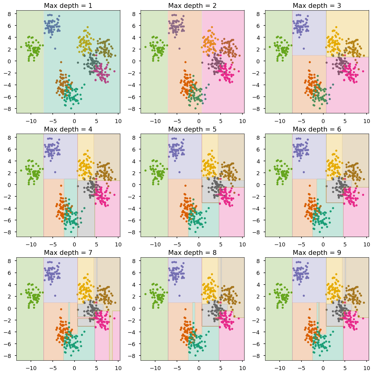
max_depth <= 3 - undefitting
max_depth <= 6 - quite good
max_depth > 6 - overfitting

Random forest¶

Lets do the same with random forests (100 trees in each forest)

from sklearn.ensemble import RandomForestClassifier as RF

# create a figure with 9 axes 3x3
fig, ax = plt.subplots(3, 3, figsize=(15,15))

# train and look at decision trees with different max depth
for max_depth in range(0, 9):
  train_and_look(RF(n_estimators=100, max_depth=max_depth + 1), X, Y,
                 ax=ax[max_depth // 3][max_depth % 3],
                 title="Max depth = {}".format(max_depth + 1))

png

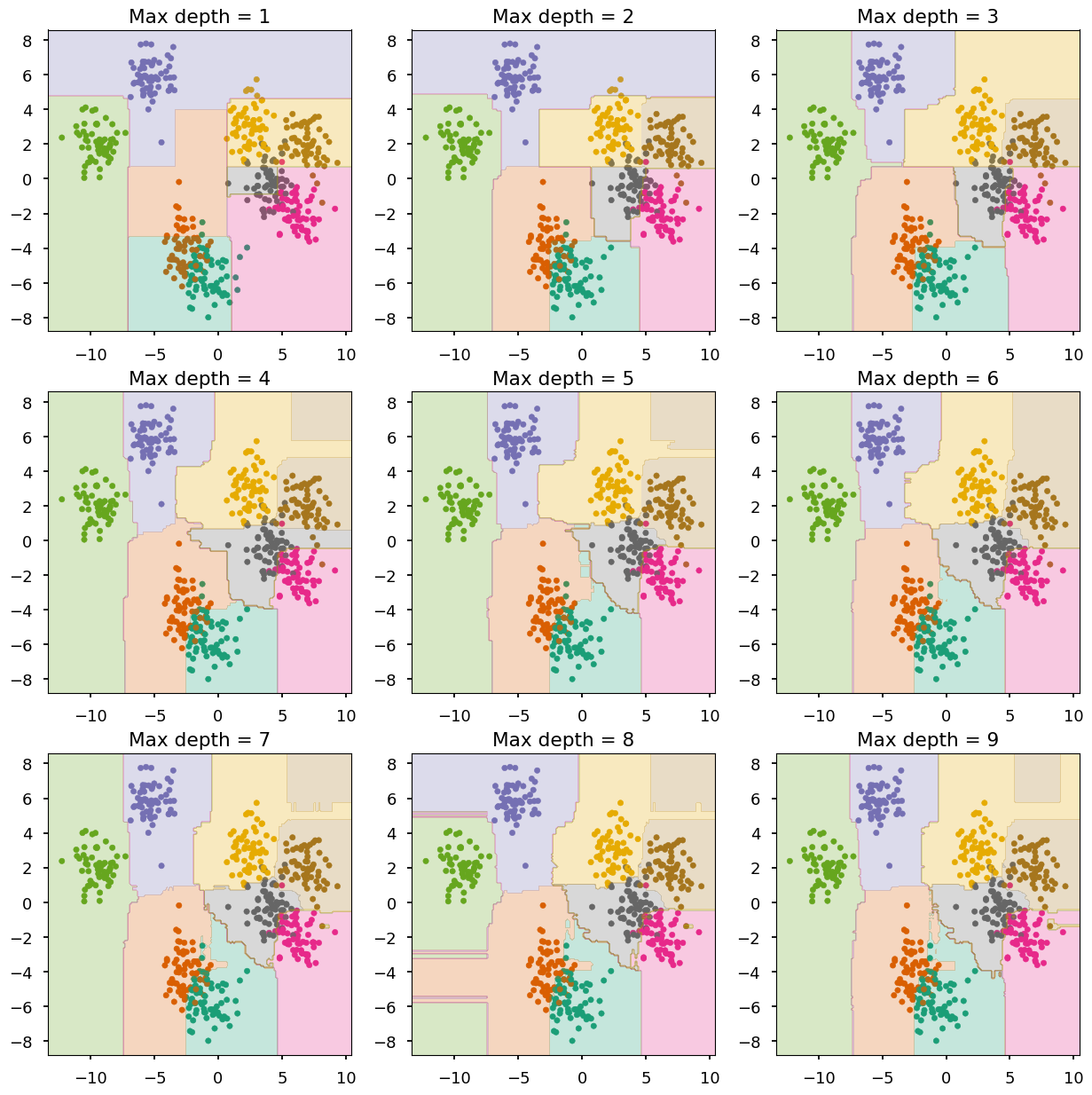
The combination of shallow trees (weak learners) does a good job
Overfitting is somehow prevented

Summary¶

The most important lesson today: bias-variance trade-off
- For the lecture easy examples are chosen so they can be visualize
- In real life problems, it is hard / impossible to determine using "bye eye" method if the model is underfitted or overfitted
- Note, that actually you should never used this method even if you think "your eye" is right - you would be surprised how it is not
- One needs a way to measure the goodnes of a model - usually mean squared error
- In practice, most people use cross-calidation technique
The biggest advantages of decision trees algoritms is that they are east to interpret (it is easy to explain even to non-experts how they work, which is not the case with e.g. deep neural networks)
Usually, decision trees are used as weak learners in ensemble learning
The most famous boosting algorithm is AdaBoost, because it is a good one and the first one. Although, there are many other boosting methods on market right now with XGBoost being one of the most popular one
As for today, deep learning has better publicity, but boosted trees are still one of the most common algorithms used in Kaggle competitions
Boosted trees are also popular among physicist and used by them as an alternative to neural networks for experimental elementary particle physics in event reconstruction procedures

	Outlook	Temperature	Humidity	Windy	Play golf
0	1	1	0	0	0
1	1	1	0	1	0
2	0	1	0	0	1
3	2	2	0	0	1
4	2	0	1	0	1
5	2	0	1	1	0
6	0	0	1	1	1
7	1	2	0	0	0
8	1	0	1	0	1
9	2	2	1	0	1
10	1	2	1	1	1
11	0	2	0	1	1
12	0	1	1	0	1
13	2	2	0	1	0

	Outlook	Temperature	Humidity	Windy	Play golf
0	1	1	0	0	0
1	1	1	0	1	0
2	0	1	0	0	1
3	2	2	0	0	1
4	2	0	1	0	1
5	2	0	1	1	0
6	0	0	1	1	1
7	1	2	0	0	0
8	1	0	1	0	1
9	2	2	1	0	1
10	1	2	1	1	1
11	0	2	0	1	1
12	0	1	1	0	1
13	2	2	0	1	0

Decision Trees¶

Graphviz¶

Installing graphviz¶

A tree example¶

Introduction¶

Decision trees¶

Example¶

ID3 and C4.5 algorithms¶

Information gain¶

Self-information¶

Information entropy¶

Information gain¶

Example¶

ID3 algorithm¶

Play Golf dataset¶

Play golf entropy¶

Play golf vs outlook¶

Results for all features¶

Root of the tree¶

Next branch¶

Last branch¶

Summary¶

C4.5 algorithm¶

Information gain ratio¶

Example¶

Continuous values¶

Example¶

Unknown parameters¶

Pruning¶

First example - step by step¶

Validation set¶

Thresholds finder¶

Feature X¶

Feature Y¶

The root¶

Branch x > 4¶

Branch x<= 8¶

Branch y > 2¶

The final tree¶

Sanity check¶

Accuracy before pruning¶

Pruning I¶

Pruning II¶

Summary¶

CART¶

Gini impurity¶

Play Golf¶

Gini impurity¶

Scikit learn¶

Regression¶

Simple example¶

Growing a tree¶

Tree: cross-validation¶

Traning dataset¶

max_depth¶

min_samples_leaf¶

min_impurity_split¶

min_impurity_decrease¶

Bias-Variance trade-off¶

Quick math¶

Basic¶

Bias and variance¶

Goodness of a model¶

Example¶

Training and test errors¶

Ensemble learning¶

Random forest¶

Intuitive / naive example¶

The algorithm¶

Boosted trees¶

AdaBoost¶

Out-of-bag error¶

Example¶

Dataset¶

Train and visualize¶

Decision tree¶

Random forest¶

Summary¶

`max_depth`¶

`min_samples_leaf`¶

`min_impurity_split`¶

`min_impurity_decrease`¶

	Outlook	Temperature	Humidity	Windy	Play golf
0	1	1	0	0	0
1	1	1	0	1	0
2	0	1	0	0	1
3	2	2	0	0	1
4	2	0	1	0	1
5	2	0	1	1	0
6	0	0	1	1	1
7	1	2	0	0	0
8	1	0	1	0	1
9	2	2	1	0	1
10	1	2	1	1	1
11	0	2	0	1	1
12	0	1	1	0	1
13	2	2	0	1	0